In [2]:
import sys; sys.version
Out[2]:
'3.5.4 |Anaconda custom (64-bit)| (default, Sep 19 2017, 08:15:17) [MSC v.1900 64 bit (AMD64)]'
In [3]:
from keras.datasets import mnist
C:\ProgramData\Anaconda3\envs\py35\lib\site-packages\h5py\__init__.py:34: FutureWarning: Conversion of the second argument of issubdtype from `float` to `np.floating` is deprecated. In future, it will be treated as `np.float64 == np.dtype(float).type`.
  from ._conv import register_converters as _register_converters
Using TensorFlow backend.
In [4]:
# images는 손글씨 숫자 이미지, labvel은 이미지의 번호
(train_images, train_labels), (test_images, test_labels) = mnist.load_data()
MNIST 데이터
In [5]:
# train: 훈련시킹 이미지들 6만개
print('train_images type: {} / len: {}'.format(type(train_images), len(train_images)))
print('train_labels type: {} / len: {}'.format(type(train_labels), len(train_labels)))
train_images type: <class 'numpy.ndarray'> / len: 60000
train_labels type: <class 'numpy.ndarray'> / len: 60000
In [6]:
# train_label : 평가 테스트용 이미지들 1만개
print('test_images type: {} / len: {}'.format(type(test_images), len(test_images)))
print('test_labels type: {} / len: {}'.format(type(test_labels), len(test_labels)))
test_images type: <class 'numpy.ndarray'> / len: 10000
test_labels type: <class 'numpy.ndarray'> / len: 10000
In [7]:
# 차원 확인:shape
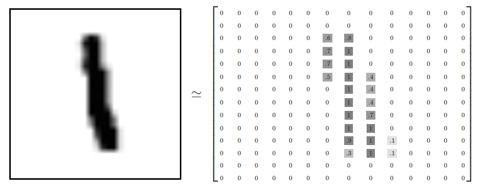
# (60000, 28, 28) -> 28x28 배열이 6만개 있다는 의미
print(train_images.shape, test_images.shape)
(60000, 28, 28) (10000, 28, 28)
- image 파일은 28x28의 배열로 이루어져 있으며 요소는 01부터 255까지 명암값으로 이루어짐.
- 이런 이미지 파일이 6만개가 있음

Matplotlib: 배열을 이미지로 출력
In [8]:
import matplotlib.pyplot as plt
In [9]:
plt.figure(figsize=(3,3))
plt.imshow(train_images[0])
plt.show()

신경망 모델을 keras로 만들기
In [10]:
from keras import models, layers

network = models.Sequential()
network.add(layers.Dense(512, activation='relu', input_shape=(28*28,)))
network.add(layers.Dense(10, activation='softmax', input_shape=(512,)))
network.compile(
    optimizer = 'adam',
    loss = 'categorical_crossentropy',
    metrics = ['accuracy'],
)
데이터 정규화
In [11]:
train_X = train_images.reshape(60000, -1)
train_X = train_X.astype('float')/ 255
test_X = test_images.reshape(10000, -1)
test_X = test_X.astype('float')/ 255
Reshapes : make output to a certain shape. - 0~255까지 있는 명암값을 255로 나누어 0~1까지의 수로 변환
In [12]:
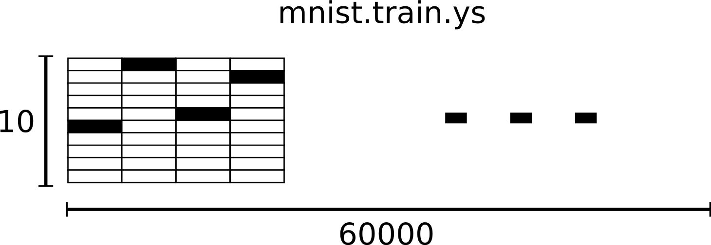
from keras.utils import to_categorical
train_Y = to_categorical(train_labels)
test_Y = to_categorical(test_labels)
In [13]:
train_Y[0] # 5
Out[13]:
array([0., 0., 0., 0., 0., 1., 0., 0., 0., 0.])
One-Hot Encoding : A vector that 1 in only one demension, 0 in the remaing demesion. - 3일 경우 [0,0,0,1,0,0,0,0,0,0,0,0] 으로 변환. - 결과적으로 tran_X는 [60000,10] 실수 배열이 된다.
머신러닝 훈련 과정
In [14]:
network.fit(train_X, train_Y, epochs=5, batch_size=128)
Epoch 1/5
60000/60000 [==============================] - 10s 172us/step - loss: 0.2695 - acc: 0.9241
Epoch 2/5
60000/60000 [==============================] - 9s 157us/step - loss: 0.1077 - acc: 0.9684
Epoch 3/5
60000/60000 [==============================] - 9s 153us/step - loss: 0.0703 - acc: 0.9795
Epoch 4/5
60000/60000 [==============================] - 9s 152us/step - loss: 0.0487 - acc: 0.9855
Epoch 5/5
60000/60000 [==============================] - 9s 151us/step - loss: 0.0360 - acc: 0.9895
Out[14]:
<keras.callbacks.History at 0x13f87b00>
테스트셋을 사용해서 평가
In [15]:
test_loss, test_acc = network.evaluate(test_X, test_Y)
10000/10000 [==============================] - 1s 96us/step
In [16]:
print('Accuracy : {:.3f}'.format(test_acc))
Accuracy : 0.981
로스 데이터
In [17]:
# test_pred: 1만개의 test_X의 예측한 값
test_pred = network.predict_classes(test_X)
import numpy as np
# correctly_predicted : 1만개의 예측된 값을 라벨값과 비교하여 참, 거짓 여부를 판단.
correctly_predicted = np.equal(test_pred, test_labels)
10000/10000 [==============================] - 1s 91us/step
In [18]:
len(test_pred), test_pred
Out[18]:
(10000, array([7, 2, 1, ..., 4, 5, 6], dtype=int64))
In [19]:
len(correctly_predicted), correctly_predicted
Out[19]:
(10000, array([ True, True, True, ..., True, True, True]))
In [20]:
# wong_predictions : 거짓(라벨값과 다름)으로 판단한 숫자들의 인덱스
wong_predictions = np.where(correctly_predicted == False)[0];
wong_predictions
Out[20]:
array([ 149,  247,  321,  340,  381,  445,  449,  582,  613,  659,  684,
        691,  740,  813,  877,  951,  956,  965, 1014, 1032, 1039, 1044,
       1112, 1156, 1178, 1182, 1194, 1226, 1232, 1242, 1247, 1260, 1289,
       1319, 1326, 1328, 1393, 1395, 1464, 1500, 1522, 1530, 1549, 1553,
       1587, 1609, 1626, 1681, 1709, 1790, 1800, 1878, 1901, 1941, 1987,
       2004, 2024, 2053, 2070, 2098, 2109, 2118, 2130, 2135, 2182, 2189,
       2272, 2293, 2387, 2488, 2534, 2597, 2607, 2648, 2654, 2713, 2720,
       2758, 2810, 2877, 2896, 2939, 2953, 3005, 3030, 3060, 3073, 3117,
       3342, 3422, 3475, 3503, 3520, 3533, 3558, 3559, 3567, 3597, 3718,
       3727, 3751, 3776, 3780, 3796, 3808, 3811, 3818, 3838, 3853, 3893,
       3906, 3926, 3941, 3976, 3985, 4065, 4078, 4116, 4199, 4248, 4289,
       4294, 4369, 4497, 4536, 4578, 4601, 4761, 4807, 4823, 4860, 4876,
       4880, 4886, 4956, 4966, 5078, 5331, 5457, 5600, 5642, 5676, 5734,
       5887, 5936, 5937, 5955, 5973, 6011, 6023, 6045, 6059, 6166, 6173,
       6555, 6571, 6574, 6576, 6597, 6598, 6625, 6651, 6783, 6847, 7216,
       7434, 7732, 7915, 8062, 8094, 8311, 8325, 8522, 8527, 9009, 9015,
       9024, 9280, 9587, 9634, 9664, 9679, 9692, 9698, 9729, 9745, 9768,
       9770, 9792, 9811, 9839, 9850, 9944], dtype=int64)
In [1]:
fig = plt.figure()
---------------------------------------------------------------------------
NameError                                 Traceback (most recent call last)
<ipython-input-1-9e2214b791fd> in <module>()
----> 1 fig = plt.figure()

NameError: name 'plt' is not defined
In [129]:
for i in range(3):
    wong_prediction = wong_predictions[i] # wong_prediction : wong_predictions에서 추출한 하나의 인덱스 번호
    plt.figure(figsize=(3,3))
    # 처음에 정의한 평가용 1만개의 이미지에 잘 못 인식한 숫자의 인덱스를 적용
    plt.imshow(test_images[wong_prediction])
    # plt.title('Predicted: {}'.format(test_pred[wong_prediction]), fontsize=30)
    plt.title('Predicted: {} / Label: {}'.format(
        test_pred[wong_prediction], test_labels[wong_prediction] ), fontsize=20)
    plt.show()


신경망 추가
In [137]:
network_deep = models.Sequential()

network_deep.add(layers.Dense(units=512, activation='relu', input_shape=(28*28,)))
network_deep.add(layers.Dense(units=256, activation='relu'))
network_deep.add(layers.Dense(units=256, activation='relu'))
network_deep.add(layers.Dense(units=10, activation='softmax'))

network_deep.compile(optimizer='adam', loss='categorical_crossentropy', metrics=['accuracy'])
In [138]:
network_deep.fit(train_X, train_Y, epochs=5, batch_size=128)
Epoch 1/5
60000/60000 [==============================] - 13s 223us/step - loss: 0.2310 - acc: 0.9322
Epoch 2/5
60000/60000 [==============================] - 13s 209us/step - loss: 0.0850 - acc: 0.9737
Epoch 3/5
60000/60000 [==============================] - 13s 211us/step - loss: 0.0546 - acc: 0.9826
Epoch 4/5
60000/60000 [==============================] - 13s 213us/step - loss: 0.0399 - acc: 0.9867
Epoch 5/5
60000/60000 [==============================] - 13s 211us/step - loss: 0.0324 - acc: 0.9895
Out[138]:
<keras.callbacks.History at 0x1e08da58>
In [139]:
_ , acc_deep = network_deep.evaluate(test_X, test_Y)
print('Accuracy of network_deep : {:.3f}'.format(acc_deep))
10000/10000 [==============================] - 1s 120us/step
Accuracy of network_deep : 0.977
클래스화
In [159]:
from keras.models import Sequential
from keras.layers import Dense
class DNN(Sequential):
    def __init__(self, input_size, output_size, *num_hidden_nodes):
        super().__init__()
        num_nodes = (*num_hidden_nodes, output_size)
        print(num_nodes)

        for idx, num_node in enumerate(num_nodes):
            activation = 'relu'
            if idx == 0:
                self.add(Dense(num_node, activation = activation, input_shape=(input_size,)))
            else:
                if idx == len(num_nodes) - 1:
                    activation = 'softmax'
                self.add(Dense(output_size, activation=activation))
        self.compile(loss='categorical_crossentropy',
                    optimizer='adam',
                    metrics=['accuracy'])
In [160]:
model = DNN(train_X.shape[1], train_Y.shape[1], 512)
(512, 10)
In [161]:
train_X[0].shape, train_Y[0].shape
Out[161]:
((784,), (10,))
In [163]:
model.fit(train_X, train_Y, epochs=5, batch_size=128)
Epoch 1/5
60000/60000 [==============================] - 10s 164us/step - loss: 0.2692 - acc: 0.9242
Epoch 2/5
60000/60000 [==============================] - 9s 151us/step - loss: 0.1088 - acc: 0.9679
Epoch 3/5
60000/60000 [==============================] - 9s 150us/step - loss: 0.0702 - acc: 0.9789
Epoch 4/5
60000/60000 [==============================] - 9s 153us/step - loss: 0.0500 - acc: 0.9852
Epoch 5/5
60000/60000 [==============================] - 9s 158us/step - loss: 0.0378 - acc: 0.9887
Out[163]:
<keras.callbacks.History at 0x1e4f5d30>
In [175]:
test_loss, test_acc = model.evaluate(test_X, test_Y)
print('Loss:{} / Acc:{}'.format(test_loss, test_acc))
10000/10000 [==============================] - 1s 98us/step
Loss:0.06835155587559566 / Acc:0.9775
In [184]:
# precidt : ML로 예측한 값.
precidt = model.predict_classes(test_X)
10000/10000 [==============================] - 1s 92us/step
In [177]:
import numpy as np
comapare_precidt = np.equal(test_precidt, test_labels) # 예측값과 라벨값과 비교
array_false = np.where(comapare_precidt == False)[0] # 비교해서 다른 것을 array_false에 추가.
len(array_false), array_false
Out[177]:
(225, array([ 115,  217,  247,  321,  340,  445,  495,  522,  527,  582,  619,
         684,  691,  720,  726,  740,  813,  846,  877,  947,  951,  956,
         965, 1014, 1039, 1055, 1112, 1156, 1173, 1182, 1194, 1226, 1232,
        1242, 1247, 1260, 1319, 1328, 1393, 1464, 1496, 1522, 1527, 1530,
        1543, 1549, 1581, 1609, 1717, 1754, 1790, 1813, 1878, 1901, 1941,
        1955, 1982, 1984, 1987, 2004, 2016, 2018, 2024, 2053, 2070, 2098,
        2109, 2118, 2130, 2135, 2182, 2272, 2293, 2387, 2414, 2447, 2488,
        2526, 2582, 2597, 2607, 2618, 2648, 2654, 2730, 2758, 2896, 2915,
        2921, 2927, 2939, 2953, 2995, 3062, 3073, 3172, 3333, 3405, 3422,
        3503, 3520, 3558, 3559, 3567, 3597, 3718, 3727, 3749, 3751, 3776,
        3780, 3818, 3853, 3893, 3906, 3941, 3968, 3976, 4065, 4075, 4078,
        4140, 4176, 4199, 4248, 4289, 4294, 4419, 4497, 4534, 4536, 4578,
        4601, 4639, 4671, 4690, 4761, 4807, 4823, 4880, 4956, 4966, 5138,
        5177, 5331, 5457, 5495, 5600, 5620, 5642, 5649, 5654, 5676, 5714,
        5734, 5749, 5835, 5858, 5887, 5936, 5937, 5955, 5972, 5973, 5982,
        5997, 6011, 6045, 6059, 6166, 6532, 6555, 6558, 6560, 6574, 6597,
        6608, 6651, 6662, 6755, 6783, 6847, 7216, 7434, 7800, 7821, 7823,
        7915, 7921, 7991, 8020, 8062, 8094, 8321, 8325, 8408, 8456, 8519,
        8522, 8527, 9009, 9015, 9019, 9024, 9071, 9280, 9534, 9587, 9634,
        9664, 9679, 9692, 9698, 9729, 9745, 9749, 9768, 9770, 9779, 9792,
        9808, 9839, 9916, 9944, 9975], dtype=int64))
In [211]:
# 잘못 인식한 숫자중 하나를 추출해서 이미지화
for i in range(20,30):
    index = array_false[i]
    select = precidt[index]
    label = test_labels[index]

    plt.imshow(test_images[index])
    plt.title('index: {}, Predict: {}, Label: {}'.format(index, select, label), fontsize=15)
    plt.show()


