はじめに
本を読むときは登場人物に関して知識がある状態で次の章に進む。
映画を見るときもそうだ。順伝播型ニューラルネットワークでは、このような時系列を考慮した記憶域を持っていない。
Recurrent Neural Networksではこういった過去の情報を考慮して未来のことを予測することができる。
今回は、実践的な時系列予測の問題をTFLearnでLSTMネットワークを構築しながら
・Recurrent Neural Networkとは何か?
・時系列データから未来を予測する方法
・LSTMとGRUを実装する方法
を解説していきますね。
解決しようとしている問題が、時系列予測の回帰モデルの問題に当てはまるとき、この方法を使えることを覚えていてほしいと思います。
Recurrent Neural Network(RNN)
Recurrent Neural Network(RNN)は、1980年代に提唱された。
ニューラルネットワークの構成がよく出来ていたにもかかわらず、ここ数年までそれほど利用されることのない技術
学習にかかる時間が現実的ではなかったようでしたが、、、
ここ数年のGPUの性能向上によって一気に普及し始めているらしいです。
時系列データを扱うRNN
RNNはニューラルネットワークのユニットに記憶域を持たせたもので、その特性上時系列データで利用される事が多い。
チャットボット・翻訳などの言語モデルや売上予測などに使われる。
個々の要素が順序を持っていて、並び方に意味のあるような問題が対象となるそうです。
簡単に説明すると文を単語に区切るとしたとします。
順序付きデータの入力は以下のように表現できます。
$x_{a}, x_{b}, x_{c},...., x_{n} $
Good morningという単語列があったとき、次の単語を予測する問題は以下の表のようになります。
| 単語 | Good | morning | ?? |
|---|---|---|---|
| 入力 | $x_{a}$ | $x_{b}$ | |
| 出力 | $y_{a}$ | $y_{b}$ |
この場合、入力値 $x_{a}$, $x_{b}$ があったときに、出力値$y_{b}$を予測することになります。
Long Short-Term Memory Networks(LSTM)
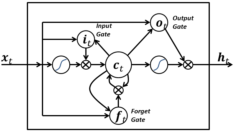
LSTM登場以前のRNNには弱点があった。長い時系列を記憶しておくことが難しかったことです。
ゲートのメカニズムを導入することで、その名の通り遠い過去のことまで覚えておくことができるようになったようです。
上図 のようにRNNセルの内部に
・入力ゲート
・出力ゲート
・忘却ゲート
が存在している。忘却ゲートがあるのは、記憶域が完全に不要になるかどうかを判断するためで、過去の影響を受けなくなったことを識別するためにあるとここでは覚えていてくださいね。
つまり、LSTMを使うべきときは遠い過去の情報まで参考にしないと予測できないような問題ということになります。
一目均衡表のデータを可視化してみる
import pandas as pd
%matplotlib inline
df = pd.read_csv('USDJPY5.txt', engine='python',usecols=[0,6],index_col='Time', parse_dates=True)
df.plot(figsize=(12, 8))
<matplotlib.axes._subplots.AxesSubplot at 0x7f5b2c005940>

まずは使用したデータの一目均衡表の可視化
import pandas as pd
%matplotlib inline
df = pd.read_csv('USDJPY5 201707260728.txt', engine='python',usecols=[0,6],index_col='Time', parse_dates=True)
df.plot(figsize=(8, 8))
<matplotlib.axes._subplots.AxesSubplot at 0x7f82a50df438>

TFLearnでRNN/LSTMネットワークを構築
LSTMに限らず、機械学習では訓練データとテストデータに分けてあとで評価できるようにしておくのが一般的ですよね。今回は67%を訓練データセット、33%をテストデータセットとして扱いました。
import numpy as np
import pandas as pd
import tflearn
import matplotlib.pyplot as plt


dataframe =pd.read_csv('USDJPY5 201707260728.txt', engine='python', usecols=[6])
dataset = dataframe.values
dataset = dataset.astype('float32')

dataset -= np.min(np.abs(dataset))
dataset /= np.max(np.abs(dataset))

def create_dataset(dataset, steps_of_history, steps_in_future):
    X, Y = [], []
    for i in range(0, len(dataset)-steps_of_history, steps_in_future):
        X.append(dataset[i:i+steps_of_history])
        Y.append(dataset[i + steps_of_history])
    X = np.reshape(np.array(X), [-1, steps_of_history, 1])
    Y = np.reshape(np.array(Y), [-1, 1])
    return X, Y

def split_data(x, y, test_size=0.1):
    pos = round(len(x) * (1 - test_size))
    trainX, trainY = x[:pos], y[:pos]
    testX, testY   = x[pos:], y[pos:]
    return trainX, trainY, testX, testY

steps_of_history = 1
steps_in_future = 1

X, Y = create_dataset(dataset, steps_of_history, steps_in_future)
trainX, trainY, testX, testY = split_data(X, Y, 0.33)

net = tflearn.input_data(shape=[None, steps_of_history, 1])
net = tflearn.lstm(net, n_units=6)
net = tflearn.fully_connected(net, 1, activation='linear')
net = tflearn.regression(net, optimizer='adam', learning_rate=0.001,
        loss='mean_square')

model = tflearn.DNN(net, tensorboard_verbose=3)
model.fit(trainX, trainY, validation_set=0.1, batch_size=1, n_epoch=100)
Training Step: 34699  | total loss: 0.00005 | time: 7.584s
| Adam | epoch: 100 | loss: 0.00005 -- iter: 346/347
Training Step: 34700  | total loss: 0.00005 | time: 8.619s
| Adam | epoch: 100 | loss: 0.00005 | val_loss: 0.00084 -- iter: 347/347
--
TensorBoardで誤差を可視化する
TFLearnはバックエンドとしてTensorFlowを使っているので、TensorFlowの可視化機構TensorBoardも使ってみました。(フローグラフとスカラーで、ちゃんと学習できてるかできていないと修正を行う為に)
model = tflearn.DNN(net, tensorboard_verbose=0)
の引数tensorboard_verboseの値を0~3にすることで可視化するログレベルを調節
0: 誤差と正解率
1: 誤差と正解率と勾配
2: 誤差と正解率と勾配と重み
3: 誤差と正解率と重みと活性度とスパース
が可視化できる。verboseのレベルを上げるとより詳細を可視化できるが、学習速度が落ちます。
$ tensorboard --logdir=/tmp/tflearn_logs
でTensorBoardを起動します。localhost:6006をブラウザからアクセスすれば起動できるはず
フローグラフやグラフ(下段)が見れたら
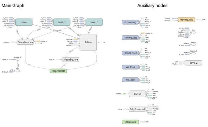
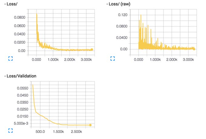
誤差が小さくなっているか、収束の速度はどうかなど見ながらハイパーパラメータを調整することができます。
時系列分析での予測精度の指標
予測や分類といった問題を解く際、設定した課題に対してどのモデルが最も適しているかを評価するための指標(評価関数)があると性能を比較しやすいので、
時系列の数値予測をする際には、その指標にRMSE、RMSLEや、MAE、MAPEといったものを使うことが多いらしいので、
以下のような関数で実装できるので、どれかを選択して試しながらやってみました。
※RMSE(Root Mean Squared Error)の場合
$$RMSE= \sqrt{ \frac{1}{N}\sum_{i=1}^{N}( y_{i}- \widehat{y}_ {i})^{2}}$$def rmse(y_pred, y_true): return np.sqrt(((y_true - y_pred) ** 2).mean())
※RMSLE(Root Mean Squared Logarithmic Error)の場合
$$RMSLE= \sqrt{ \frac{1}{N}\sum_{i=1}^{N}( log(y_{i}+1)-log( y^{t}_{i}+1))^{2}}$$def rmsle(y_pred, y_true): return np.sqrt(np.square(np.log(y_true + 1) - np.log(y_pred + 1)).mean())
※MAE(Mean Absolute Error)の場合
$$MAE= \frac{1}{N}\sum_{i=1}^{N} \mid y_{i}- \widehat{y}_ {i}\mid $$def mae(y_pred, y_true): return np.mean(np.abs((y_true - y_pred)))
※ MAPE(Mean Absolute Percentage Error)の場合
$$MAPE= \frac{100}{N}\sum_{i=1}^{N} \frac{ \mid y_{i}- \widehat{y}_ {i}\mid }{ y_{i} } $$def mape(y_pred, y_true): return np.mean(np.abs((y_true - y_pred) / y_true)) * 100
※ 結果は別資料参照
import numpy as np
import pandas as pd
import tflearn
import matplotlib.pyplot as plt
%matplotlib inline

dataframe =pd.read_csv('USDJPY5 201707260728.txt', engine='python', usecols=[6])
dataset = dataframe.values
dataset = dataset.astype('float32')

dataset -= np.min(np.abs(dataset))
dataset /= np.max(np.abs(dataset))

def create_dataset(dataset, steps_of_history, steps_in_future):
    X, Y = [], []
    for i in range(0, len(dataset)-steps_of_history, steps_in_future):
        X.append(dataset[i:i+steps_of_history])
        Y.append(dataset[i + steps_of_history])
    X = np.reshape(np.array(X), [-1, steps_of_history, 1])
    Y = np.reshape(np.array(Y), [-1, 1])
    return X, Y

def split_data(x, y, test_size=0.1):
    pos = round(len(x) * (1 - test_size))
    trainX, trainY = x[:pos], y[:pos]
    testX, testY   = x[pos:], y[pos:]
    return trainX, trainY, testX, testY

steps_of_history = 1
steps_in_future = 1

X, Y = create_dataset(dataset, steps_of_history, steps_in_future)
trainX, trainY, testX, testY = split_data(X, Y, 0.33)

net = tflearn.input_data(shape=[None, steps_of_history, 1])
net = tflearn.lstm(net, n_units=6)
net = tflearn.fully_connected(net, 1, activation='linear')
net = tflearn.regression(net, optimizer='adam', learning_rate=0.001,
        loss='mean_square')

model = tflearn.DNN(net, tensorboard_verbose=0)
model.fit(trainX, trainY, validation_set=0.1, batch_size=1, n_epoch=150)

# 可視化するプログラム
train_predict = model.predict(trainX)
test_predict = model.predict(testX)

train_predict_plot = np.empty_like(dataset)
train_predict_plot[:, :] = np.nan
train_predict_plot[steps_of_history:len(train_predict)+steps_of_history, :] = \
        train_predict

test_predict_plot = np.empty_like(dataset)
test_predict_plot[:, :] = np.nan
test_predict_plot[len(train_predict)+steps_of_history:len(dataset), :] = \
        test_predict

plt.figure(figsize=(8, 8))
plt.title('History={} Future={}'.format(steps_of_history, steps_in_future))
plt.plot(dataset)
plt.plot(train_predict_plot)
plt.plot(test_predict_plot)
plt.savefig('passenger.png')
Training Step: 52049  | total loss: 0.00007 | time: 2.760s
| Adam | epoch: 150 | loss: 0.00007 -- iter: 346/347
Training Step: 52050  | total loss: 0.00006 | time: 3.774s
| Adam | epoch: 150 | loss: 0.00006 | val_loss: 0.00018 -- iter: 347/347
--

訓練データが少ない割には似通ったグラフがプロットされました。
Window幅を変えてみる
直近数回分のデータを入力値として、次の乗客数を予測することもできる。つまり、, , の値を入力値として、の値を予測する。
入力のWindow幅を3に変更してみよう。
steps_of_history = 3
として実行してみる。
import numpy as np
import pandas as pd
import tflearn
import matplotlib.pyplot as plt
%matplotlib inline


dataframe =pd.read_csv('USDJPY5 201707260728.txt', engine='python', usecols=[6])
dataset = dataframe.values
dataset = dataset.astype('float32')

dataset -= np.min(np.abs(dataset))
dataset /= np.max(np.abs(dataset))

def create_dataset(dataset, steps_of_history, steps_in_future):
    X, Y = [], []
    for i in range(0, len(dataset)-steps_of_history, steps_in_future):
        X.append(dataset[i:i+steps_of_history])
        Y.append(dataset[i + steps_of_history])
    X = np.reshape(np.array(X), [-1, steps_of_history, 1])
    Y = np.reshape(np.array(Y), [-1, 1])
    return X, Y

def split_data(x, y, test_size=0.1):
    pos = round(len(x) * (1 - test_size))
    trainX, trainY = x[:pos], y[:pos]
    testX, testY   = x[pos:], y[pos:]
    return trainX, trainY, testX, testY

steps_of_history = 3
steps_in_future = 1

X, Y = create_dataset(dataset, steps_of_history, steps_in_future)
trainX, trainY, testX, testY = split_data(X, Y, 0.33)

net = tflearn.input_data(shape=[None, steps_of_history, 1])
net = tflearn.lstm(net, n_units=6)
net = tflearn.fully_connected(net, 1, activation='linear')
net = tflearn.regression(net, optimizer='adam', learning_rate=0.001,
        loss='mean_square')

model = tflearn.DNN(net, tensorboard_verbose=0)
model.fit(trainX, trainY, validation_set=0.1, batch_size=1, n_epoch=150)

train_predict = model.predict(trainX)
test_predict = model.predict(testX)

train_predict_plot = np.empty_like(dataset)
train_predict_plot[:, :] = np.nan
train_predict_plot[steps_of_history:len(train_predict)+steps_of_history, :] = \
        train_predict

test_predict_plot = np.empty_like(dataset)
test_predict_plot[:, :] = np.nan
test_predict_plot[len(train_predict)+steps_of_history:len(dataset), :] = \
        test_predict

plt.figure(figsize=(8, 8))
plt.title('History={} Future={}'.format(steps_of_history, steps_in_future))
plt.plot(dataset)
plt.plot(train_predict_plot)
plt.plot(test_predict_plot)
plt.savefig('passenger.png')
Training Step: 51899  | total loss: 0.00011 | time: 2.538s
| Adam | epoch: 150 | loss: 0.00011 -- iter: 345/346
Training Step: 51900  | total loss: 0.00010 | time: 3.558s
| Adam | epoch: 150 | loss: 0.00010 | val_loss: 0.00017 -- iter: 346/346
--

あまり改善されていない
import numpy as np
import pandas as pd
import tflearn
import matplotlib.pyplot as plt
%matplotlib inline

dataframe = pd.read_csv('USDJPY5 201707260728.txt', engine='python', usecols=[6])
dataset = dataframe.values
dataset = dataset.astype('float32')

dataset -= np.min(np.abs(dataset))
dataset /= np.max(np.abs(dataset))

def create_dataset(dataset, steps_of_history, steps_in_future):
    X, Y = [], []
    for i in range(0, len(dataset)-steps_of_history, steps_in_future):
        X.append(dataset[i:i+steps_of_history])
        Y.append(dataset[i + steps_of_history])
    X = np.reshape(np.array(X), [-1, steps_of_history, 1])
    Y = np.reshape(np.array(Y), [-1, 1])
    return X, Y

def split_data(x, y, test_size=0.1):
    pos = round(len(x) * (1 - test_size))
    trainX, trainY = x[:pos], y[:pos]
    testX, testY   = x[pos:], y[pos:]
    return trainX, trainY, testX, testY

steps_of_history = 1
steps_in_future = 1

X, Y = create_dataset(dataset, steps_of_history, steps_in_future)
trainX, trainY, testX, testY = split_data(X, Y, 0.33)

net = tflearn.input_data(shape=[None, steps_of_history, 1])
net = tflearn.gru(net, n_units=6)
net = tflearn.fully_connected(net, 1, activation='linear')
net = tflearn.regression(net, optimizer='adam', learning_rate=0.001,
        loss='mean_square')

model = tflearn.DNN(net, tensorboard_verbose=0)
model.fit(trainX, trainY, validation_set=0.1, batch_size=1, n_epoch=100)

train_predict = model.predict(trainX)
test_predict = model.predict(testX)

train_predict_plot = np.empty_like(dataset)
train_predict_plot[:, :] = np.nan
train_predict_plot[steps_of_history:len(train_predict)+steps_of_history, :] = \
        train_predict

test_predict_plot = np.empty_like(dataset)
test_predict_plot[:, :] = np.nan
test_predict_plot[len(train_predict)+steps_of_history:len(dataset), :] = \
        test_predict

plt.figure(figsize=(8, 8))
plt.title('History={} Future={}'.format(steps_of_history, steps_in_future))
plt.plot(dataset)
plt.plot(train_predict_plot)
plt.plot(test_predict_plot)
plt.savefig('passenger.png')
Training Step: 34699  | total loss: 0.00009 | time: 1.689s
| Adam | epoch: 100 | loss: 0.00009 -- iter: 346/347
Training Step: 34700  | total loss: 0.00010 | time: 2.704s
| Adam | epoch: 100 | loss: 0.00010 | val_loss: 0.00022 -- iter: 347/347
--

こちらは随分と推定値が実際の値に近くなったように見える。
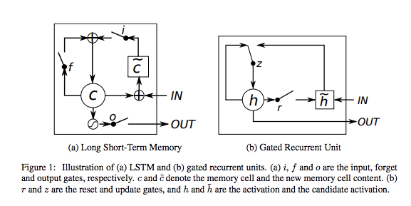
GRUの層を増やしてみる
GRUの層の数を増やしてみよう。return_seqパラメーターをTrueにして2つ繋げてみる。
net = tflearn.gru(net, n_units=6)
の部分を
net = tflearn.gru(net, n_units=6, return_seq=True) net = tflearn.gru(net, n_units=6) とするだけでいい。
実行してみよう。
import numpy as np
import pandas as pd
import tflearn
import matplotlib.pyplot as plt
%matplotlib inline

dataframe = pd.read_csv('USDJPY5 201707260728.txt', engine='python', usecols=[6])
dataset = dataframe.values
dataset = dataset.astype('float32')

dataset -= np.min(np.abs(dataset))
dataset /= np.max(np.abs(dataset))

def create_dataset(dataset, steps_of_history, steps_in_future):
    X, Y = [], []
    for i in range(0, len(dataset)-steps_of_history, steps_in_future):
        X.append(dataset[i:i+steps_of_history])
        Y.append(dataset[i + steps_of_history])
    X = np.reshape(np.array(X), [-1, steps_of_history, 1])
    Y = np.reshape(np.array(Y), [-1, 1])
    return X, Y

def split_data(x, y, test_size=0.1):
    pos = round(len(x) * (1 - test_size))
    trainX, trainY = x[:pos], y[:pos]
    testX, testY   = x[pos:], y[pos:]
    return trainX, trainY, testX, testY

steps_of_history = 3
steps_in_future = 1

X, Y = create_dataset(dataset, steps_of_history, steps_in_future)
trainX, trainY, testX, testY = split_data(X, Y, 0.33)

net = tflearn.input_data(shape=[None, steps_of_history, 1])
net = tflearn.gru(net, n_units=6, return_seq=True)
net = tflearn.gru(net, n_units=6)
net = tflearn.fully_connected(net, 1, activation='linear')
net = tflearn.regression(net, optimizer='adam', learning_rate=0.001,
        loss='mean_square')

model = tflearn.DNN(net, tensorboard_verbose=0)
model.fit(trainX, trainY, validation_set=0.1, batch_size=1, n_epoch=100)

train_predict = model.predict(trainX)
test_predict = model.predict(testX)

train_predict_plot = np.empty_like(dataset)
train_predict_plot[:, :] = np.nan
train_predict_plot[steps_of_history:len(train_predict)+steps_of_history, :] = \
        train_predict

test_predict_plot = np.empty_like(dataset)
test_predict_plot[:, :] = np.nan
test_predict_plot[len(train_predict)+steps_of_history:len(dataset), :] = \
        test_predict

plt.figure(figsize=(8, 8))
plt.title('History={} Future={}'.format(steps_of_history, steps_in_future))
plt.plot(dataset)
plt.plot(train_predict_plot)
plt.plot(test_predict_plot)
plt.savefig('passenger.png')
Training Step: 34599  | total loss: 0.00019 | time: 2.242s
| Adam | epoch: 100 | loss: 0.00019 -- iter: 345/346
Training Step: 34600  | total loss: 0.00017 | time: 3.261s
| Adam | epoch: 100 | loss: 0.00017 | val_loss: 0.00056 -- iter: 346/346
--

LSTM学習のコツ
LSTMのパラメーターはどのように決定すればいいのだろうか?
わかるLSTMという記事に参考になる記述があったので紹介しますね。
まず、学習率の設定は何においても重要になります。データセットによって大きく傾向が異なりますが、予測誤差が一気に改善する特異な地点が存在することがわかります。
論文中ではまず高い学習率(1程度)から始めて、性能の改善が停止するたびに10で割る大雑把な探索が推奨されています。
一方で、隠れ層の数については非常にわかりやすい傾向が出ています。
期待通り、隠れ層の数を増やせば増やすほど性能は改善しますが、そのトレードオフとして実行時間が増加します。
なお、図表に示されてはいませんが、モーメンタムの値は今回の解析では値の設定による性能の変化はなかったと報告されています。
BPTTの打ち切りステップ数についての言及はこの論文ではありませんでしたが、直感的には獲得したい長期依存の長さとタスクの実行時間とのバランスを取るのが標準的な戦略だと思われます。
まとめ
サンプル数は少なかったが、実践的な例題を通してLSTMからGRUまで試してみました。
RNNを使うことで、順伝播型ニューラルネットワークでは出来なかった順序列を扱うようなニューラルネットワークも構築することができる。
時系列予測や言語モデルなどにもすでに応用されていて、新しいニューラルネットのアーキテクチャも次々と提案されるようになった。
今後もまだまだ発展するだろうと感じている。
参考
Time Series Prediction with LSTM Recurrent Neural Networks in Python with Keras