
- rafael AT rebelliondefense.com
- aaron AT rebelliondefense.com
- shay AT rebelliondefense.com
- tom AT rebelliondefense.com
- jackie AT rebelliondefense.com
Table of Contents
- Introduction
- What is Approximate Nearest Neighbor Search?
- Obtaining Vectors and Distance Functions From Datasets
- Applications of Approximate Nearest Neighbor Search
- Considerations when selecting an Approximate Nearest Neighbor Search
- Hands-On
- Installing NGT and HIPCML
- Visualizing the Connections in a Dataset as a Graph
- Manifold Learning with UMAP
- Graph Clustering
- Conclusion
- Contact
Introduction
At Rebellion, we are constantly leveraging techniques to scalably organize large datasets to create insights to achieve operations goals for our customers. A common problem people face is to group data and discover relationships that would overwise go unnoticed. One way to this is by transforming your initially confusing sea of data into a nice clear map. Using this new representation, we can easily ask questions such as, "Give me things similar to this?", "What is the most different thing from this other things?", "What is unique?"
To start this process, we need data. From the data, we derive a list of numerical observations. Usually, this is called a vector or matrix. An image, for example, is just a matrix, after all. Network traffic is another example, where we isolate certain observations and want to understand how our network traffic evolves.
Usually, our first pass at creating a numerical representation is very complicated and redundant. It is hard to see any patterns. This is where the techniques we describe in this post can help.
What is Approximate Nearest Neighbor Search?
Say we have a vector $q \in \mathbb{R}^n$ and a collection vectors, $V \subset \mathbb{R}^n$, and we would like to know which vectors in $V$ are "neighbors" of $q$. We can define "neighbors" in a few ways. We can say vectors in $V$ that are at most $\epsilon >= 0$ distance way from $q$ are its neighbors. We can also ask for the $k$ nearest points from $V$ to $q$. These kinds of neighbors are known as $\epsilon$-neighbors and $k$-nearest neighbors.
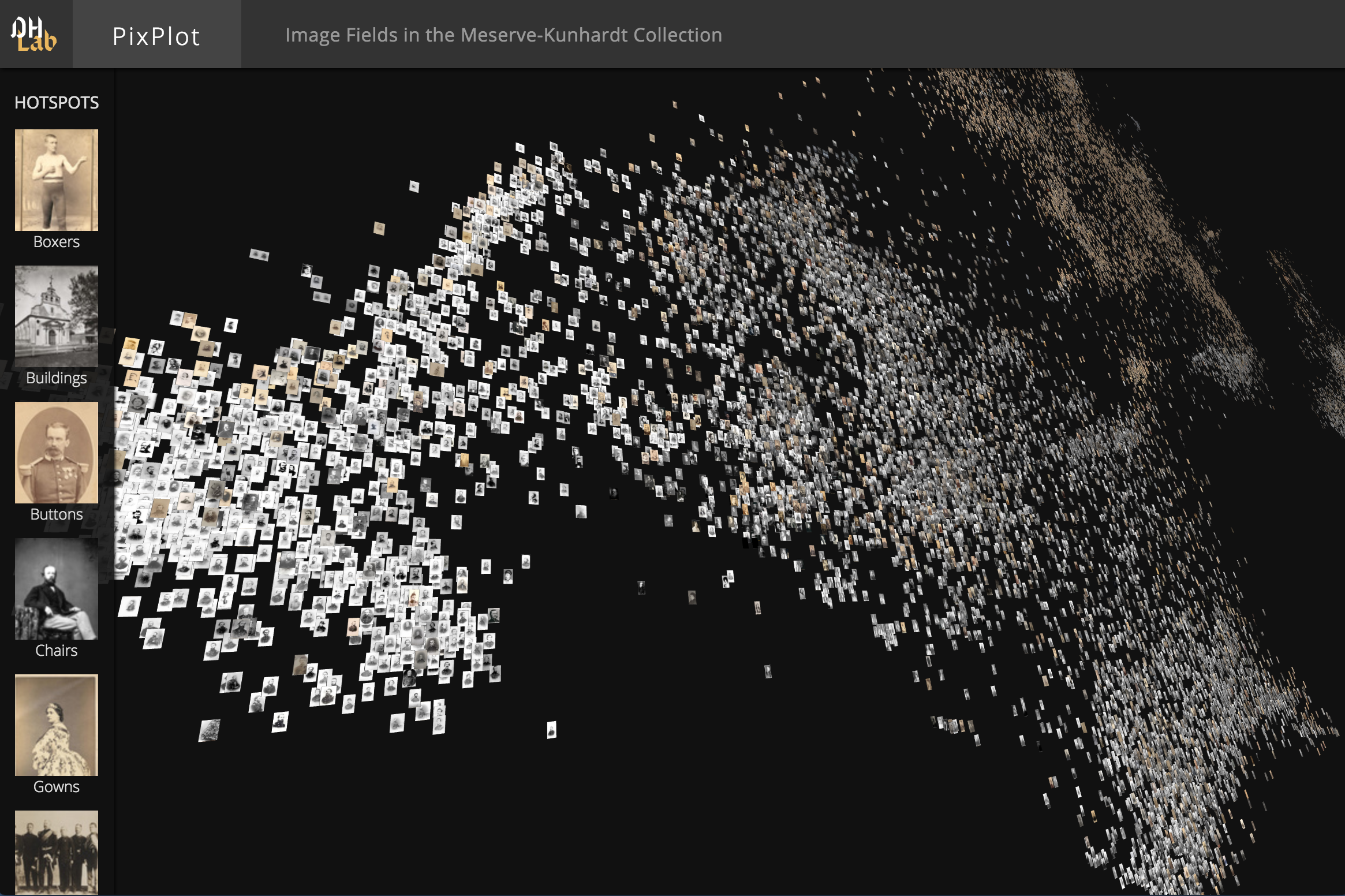
However, we can do more than query individual vectors for nearest neighbors. We can also summarize entire datasets using a network representation. If we consider the nodes to be the vectors and edges to be drawn if two vectors are in the same neighborhood, we can visualize, explore, and isolate relational patterns across the entire dataset. Good examples of this using graph summarization of vector data are Yale Digital Humanities Lab Team's pix-plot and Google's Projector.
Unfortunately, performing an exact nearest neighbor search using simple methods has a runtime of $O(n|V|)$ where $|V|$ is how many vectors you are considering, and $n$ is the dimension of each vector. In practice, there is a tradeoff between the speed of retrieval and the accuracy of neighbors returned.
Obtaining Vectors and Distance Functions From Datasets
While some datasets are already vectors and have natural notion distance, many datasets do not. A vector representation of data is a numerical representation that helps capture some aspect of the meaning of the data. Datasets made-up of words from natural language do not have a clear vector representation and distance. In these cases, neural networks can transform words into vectors. An entire field of Machine Learning called representation learning can be seen as a methodical attempt of transforming raw data into vectors that have a meaningful notion of distance. For example, Facebook's fasttext and Google's BERT are examples of techniques of turning natural language into a vector representation. Another way to turn words into vectors is through so-called context vectors.
In the case of images, vectors could be created by taking second to the last layer of a pre-trained neural network, such as Inception. Techniques include using autoencoders or flattening the RGB matrices and concatenating them together to form a vector.
Applications of Approximate Nearest Neighbor Search
There are two general uses of the nearest neighbor search. One application is to search a database of vectors to retrieve similar vectors to the query vector. This type of usage is a local estimate to determine the closest items from the perspective of a single vector. Recommendation engines and georegistration are example applications that can be powered by approximate nearest neighbor search.
Other applications need to estimate how the entire dataset is globally related. In these use-cases, a graph is created by transforming all the vectors into nodes and edges where an edge connects two vectors if the vectors are neighbors. While this graph forgets the vectors' exact values, it maintains the relationship between the vectors and is a scalable and sparse representation of the topology. Creating this graph is often the first step in applications such as dimensionality reduction, where one can define neighbors based on either k-nearest neighbor graph or $\epsilon$-neighborhood graph. UMAP, for example, creates a k-nearest neighbor graph using the nn descent algorthim.
Considerations when selecting an Approximate Nearest Neighbor Search
An excellent place to learn about the performance of different ANN libraries is using Martin Aumueller's and Erik Bernhardsson's ann-benchmark. Here is an example performance assessment from 2019-06-10 showing the tradeoff between the speed of retrieval and accuracy 784-dimensional vectors from Fashion MNIST:

Another consideration is the deployment of the nearest neighbor library and if there is a serving front-end that is useable within your existing infrastructure. While many backend libraries will perform an approximate nearest neighbor search, not all of them have an abstracted API that is easy for external clients to use the library.
Here is a chart outlining which ANN libraries have built RPC for serving requests:
| Library | Serving Layer | Technique | Hardware Acceleration | Organization Usage |
|---|---|---|---|---|
| NGT | GRPC | ANNG | None | Yahoo |
| ANNOY | None | Random Projections | None | Spotify |
| Faiss | None | Many | GPU | |
| NMSLIB | HTTP | Many | None | Amazon |
| SPTAG | Custom TCP Protocol | Many | None | Microsoft |
| Scann | None | Many | AVX2 |
As we outlined above, there are two broad applications of approximate nearest neighbor search. The critical question is, "what type of intermediate results does the approximate nearest neighbor search library expose in a performant manner?". A recommendation engine or image search engine may only need to make local queries to the approximate nearest neighbor library. Dimensionality reduction, on the other hand, will process an initial graph summary of the data. While you can create the graph by making subsequent calls to the library one vector at a time, it can be more convenient and faster if the library can return the graph. NGT, for example, allows you to create multiple graphs from datasets of vectors. Let's see how we do that in the next section.
Installing NGT and HIPMCL
We will be using a development branch of NGT located at https://github.com/masajiro/NGT/tree/devel . Let's pull it down and install it.
git clone https://github.com/masajiro/NGT.git NGT_DEV cd NGT_DEV/ git checkout devel /usr/bin/ruby -e "$(curl -fsSL https://raw.githubusercontent.com/Homebrew/install/master/install)" brew install cmake brew install gcc@9 export CXX=/usr/local/bin/g++-9 export CC=/usr/local/bin/gcc-9 mkdir build cd build cmake .. make make install
Running the ngt command should now return:
Usage : ngt command [options] index [data] command : info create search remove append export import prune reconstruct-graph optimize-search-parameters optimize-#-of-edges repair Version : 1.11.5
Summarizing Connections in a Dataset as a Graph
In this example, we are going to work with word vectors from Facebook and explore how the model is relating words to one another. First, we download the data and create 4 different graphs: ANNG, Refined ANNG, KNNG, CKNNG.
curl -O https://dl.fbaipublicfiles.com/fasttext/vectors-english/wiki-news-300d-1M-subword.vec.zip
unzip wiki-news-300d-1M-subword.vec.zip
tail -n +2 wiki-news-300d-1M-subword.vec | cut -d " " -f 2- > wiki-news-300d-1M-subword.ssv
Insert objects and build an initial index.
ngt create -d 100 -o f -E 15 -D c anng wiki-news-300d-1M-subword.ssv
Optimize search parameters to enable the expected accuracy for search
ngt optimize-search-parameters anng
Export an ANNG
ngt export-graph anng > anng.graph
reconstruct a refined ANNG with an expected accuracy is 0.95
ngt refine-anng -a 0.95 anng refined-anng ranng
Export a refined ANNG
ngt export-graph refined-anng > refined-anng.graph
Export an approximate KNNG (k=15)
ngt export-graph -k 15 refined-anng > approximate-knng.graph
Export an approximate CKNNG (k=15)
ngt reconstruct-cknng -k 15 -d 1 ranng cknng
ngt export-graph cknng > approximate-cknng.graph
Plotting a million vertex graph is a little overwhelming (that is part of the usefulness of UMAP we which we discuss next). Let us plot a simpler graph to get an intuition for what the graph summary offers us. I created a KNN graph from the Iris dataset. Note the colors correspond to different flows. The graph creation step did not use the flower's identity, just measurements of the width and length of the petals and sepals. We can see the clear separation just by looking at the graph:

Manifold Learning with UMAP
Now that we have our graphs, we can start to do analysis over. In this first example, we will apply UMAP to our KNN graph.
from umap.umap_ import compute_membership_strengths, smooth_knn_dist, make_epochs_per_sample, simplicial_set_embedding, find_ab_params
import scipy


# Load graphs created by NGT
def load_knn_graph(ngt_graph):
    knn_indices = []
    knn_dist = []

    nodes_with_no_edges = set()
    with open(ngt_graph, "r") as f:
        while True:
            line = f.readline().strip("\n").strip()
            if not line:
                break
            token = line.split("\t")
            start_node = int(token[0])
            end_nodes = token[1:]

            if end_nodes == []:
                nodes_with_no_edges.add(start_node)
                continue

            knn_entry = []
            knn_entry_dist = []
            for ith in range(0, len(end_nodes), 2):
                try:
                    end_node = int(end_nodes[ith])
                except Exception as e:
                    nodes_with_no_edges.add(start_node)
                    continue
                knn_entry.append(end_node)
                weight = float(end_nodes[ith+1])
                knn_entry_dist.append(weight)
            knn_indices.append(knn_entry)
            knn_dist.append(knn_entry_dist)


    return np.array(knn_indices), np.array(knn_dist)


def knn_fuzzy_simplicial_set(knn_indices, knn_dists, local_connectivity, set_op_mix_ratio, apply_set_operations):

    n_samples = knn_indices.shape[0]
    n_neighbors = knn_indices.shape[1]

    knn_dists = knn_dist.astype(np.float32)

    sigmas, rhos = smooth_knn_dist(
        knn_dists, float(n_neighbors), local_connectivity=float(local_connectivity),
    )

    rows, cols, vals = compute_membership_strengths(
        knn_indices, knn_dists, sigmas, rhos
    )

    result = scipy.sparse.coo_matrix(
        (vals, (rows, cols)), shape=(n_samples, n_samples)
    )
    result.eliminate_zeros()

    if apply_set_operations:
        transpose = result.transpose()

        prod_matrix = result.multiply(transpose)

        result = (
            set_op_mix_ratio * (result + transpose - prod_matrix)
            + (1.0 - set_op_mix_ratio) * prod_matrix
        )

    result.eliminate_zeros()

    return result, sigmas, rhos


def transform(graph, metric="l2", n_components = 2, n_epochs = 500, spread=1.0, min_dist = 0.0, initial_alpha=1.0, negative_sample_rate=5, repulsion_strength=7):
    graph = graph.tocoo()
    graph.sum_duplicates()
    n_vertices = graph.shape[1]

    if n_epochs <= 0:
        # For smaller datasets we can use more epochs
        if graph.shape[0] <= 10000:
            n_epochs = 500
        else:
            n_epochs = 200

    graph.data[graph.data < (graph.data.max() / float(n_epochs))] = 0.0
    graph.eliminate_zeros()

    epochs_per_sample = make_epochs_per_sample(graph.data, n_epochs)

    head = graph.row
    tail = graph.col
    weight = graph.data

    a, b = find_ab_params(spread, min_dist)

    emebedding = simplicial_set_embedding(None, graph, n_components=2, initial_alpha=1.0, a=a, b=b, gamma=repulsion_strength, negative_sample_rate=negative_sample_rate, random_state=np.random, metric=metric, metric_kwds=None, verbose=True, parallel=True, n_epochs=n_epochs, init="random")

    return emebedding
import numpy as np

# Example data for Iris can be found here: https://github.com/lmcinnes/umap/files/4921774/approximate-knng.txt
knn_indices, knn_dist = load_knn_graph("approximate-knng.txt")

knn_indices = knn_indices - 1

local_connectivity = 1
apply_set_operations = True
set_op_mix_ratio=1.0

graph, sigmas, rhos = knn_fuzzy_simplicial_set(knn_indices, knn_dist, local_connectivity, set_op_mix_ratio, apply_set_operations)

emebedding = transform(graph, metric="l2", n_components = 2, n_epochs = 500, spread=1.0, min_dist = 0.0, initial_alpha=1.0, negative_sample_rate=5, repulsion_strength=7)
Let's see what our embedding looks like. I have already plotted two embeddings, one for the word vectors and another one for the graph we created from the iris dataset.
import matplotlib.pyplot as plt

image = plt.imread('wordvector_embedding.png')
plt.imshow(image);

image = plt.imread('iris_umap.png')
plt.axis('off')
plt.imshow(image);

Graph Clustering
In this section, we show how to cluster the graphs created above using HipMCL. HipMCL is a high-performance implementation of Markov clustering algorithm from the Department of Energy. After you install HipMCL you can run it on one of the graphs created below using:
./bin/hipmcl -M approximate-knng.triples -I 2 -per-process-mem 20 -o knng_clusters.txt
You can also the following Python library to compute the clustering: https://github.com/GuyAllard/markov_clustering . When we cluster the graph above, we see that we recover three groups, each one referring to one of the three plants in the dataset.

Conclusion
In conclusion, we have shown how to summarize data using graphs and to use these graphs to create embeddings with UMAP as well as cluster data. By isolating the graph construction from the embedding, we can create more modular systems and iterate faster on different graphs.