import numpy as np
import pandas as pd
import matplotlib.pyplot as plt
import seaborn as sns

import warnings
warnings.filterwarnings("ignore")
warnings.warn("this will not show")

plt.rcParams["figure.figsize"] = (10,6)

sns.set_style("whitegrid")
pd.set_option('display.float_format', lambda x: '%.3f' % x)

# Set it None to display all rows in the dataframe
# pd.set_option('display.max_rows', None)

# Set it to None to display all columns in the dataframe
pd.set_option('display.max_columns', None)
print("%s" % ("hello", ))
hello
print("{arg3:>20}|{arg2:^10}|{arg2:5}".format(arg1="hello", arg2="world", arg3="python"))
python| world |world
from IPython.display import Image
Image(url= "https://static1.squarespace.com/static/5006453fe4b09ef2252ba068/5095eabce4b06cb305058603/5095eabce4b02d37bef4c24c/1352002236895/100_anniversary_titanic_sinking_by_esai8mellows-d4xbme8.jpg")

Exploratory Data Analysis (EDA) on Titanic Dataset
¶Aim
Applying Exploratory Data Analysis (EDA) and preparing the data to implement the Machine Learning Algorithms
- Analyzing the features according to survival status (target feature)
- Preparing data to create a model that will predict the survival status of people (So the "survive" feature is the target feature)
Let's read the data from file
# "C:/Users/tuseb.000/Desktop/Cohorts/DE-DS Cohort-01/DAwPY/titanic_train.csv"

df = pd.read_csv("titanic.csv", sep="\t")
df
| PassengerId | Survived | Pclass | Name | Sex | Age | SibSp | Parch | Ticket | Fare | Cabin | Embarked | |
|---|---|---|---|---|---|---|---|---|---|---|---|---|
| 0 | 1 | 0 | 3 | Braund, Mr. Owen Harris | male | 22.000 | 1 | 0 | A/5 21171 | 7.250 | NaN | S |
| 1 | 2 | 1 | 1 | Cumings, Mrs. John Bradley (Florence Briggs Th... | female | 38.000 | 1 | 0 | PC 17599 | 71.283 | C85 | C |
| 2 | 3 | 1 | 3 | Heikkinen, Miss. Laina | female | 26.000 | 0 | 0 | STON/O2. 3101282 | 7.925 | NaN | S |
| 3 | 4 | 1 | 1 | Futrelle, Mrs. Jacques Heath (Lily May Peel) | female | 35.000 | 1 | 0 | 113803 | 53.100 | C123 | S |
| 4 | 5 | 0 | 3 | Allen, Mr. William Henry | male | 35.000 | 0 | 0 | 373450 | 8.050 | NaN | S |
| ... | ... | ... | ... | ... | ... | ... | ... | ... | ... | ... | ... | ... |
| 151 | 152 | 1 | 1 | Pears, Mrs. Thomas (Edith Wearne) | female | 22.000 | 1 | 0 | 113776 | 66.600 | C2 | S |
| 152 | 153 | 0 | 3 | Meo, Mr. Alfonzo | male | 55.500 | 0 | 0 | A.5. 11206 | 8.050 | NaN | S |
| 153 | 154 | 0 | 3 | van Billiard, Mr. Austin Blyler | male | 40.500 | 0 | 2 | A/5. 851 | 14.500 | NaN | S |
| 154 | 155 | 0 | 3 | Olsen, Mr. Ole Martin | male | NaN | 0 | 0 | Fa 265302 | 7.312 | NaN | S |
| 155 | 156 | 0 | 1 | Williams, Mr. Charles Duane | male | 51.000 | 0 | 1 | PC 17597 | 61.379 | NaN | C |
156 rows × 12 columns
pwd
'/Users/kirbyurner/Documents/clarusway_data_analysis/DAwPy_S12_(Recap-EDA on Titanic Dataset)'
Let's understand the data
df.head(5)
| PassengerId | Survived | Pclass | Name | Sex | Age | SibSp | Parch | Ticket | Fare | Cabin | Embarked | |
|---|---|---|---|---|---|---|---|---|---|---|---|---|
| 0 | 1 | 0 | 3 | Braund, Mr. Owen Harris | male | 22.000 | 1 | 0 | A/5 21171 | 7.250 | NaN | S |
| 1 | 2 | 1 | 1 | Cumings, Mrs. John Bradley (Florence Briggs Th... | female | 38.000 | 1 | 0 | PC 17599 | 71.283 | C85 | C |
| 2 | 3 | 1 | 3 | Heikkinen, Miss. Laina | female | 26.000 | 0 | 0 | STON/O2. 3101282 | 7.925 | NaN | S |
| 3 | 4 | 1 | 1 | Futrelle, Mrs. Jacques Heath (Lily May Peel) | female | 35.000 | 1 | 0 | 113803 | 53.100 | C123 | S |
| 4 | 5 | 0 | 3 | Allen, Mr. William Henry | male | 35.000 | 0 | 0 | 373450 | 8.050 | NaN | S |
Explanations about data from Kaggle
| Variable | Definition | Key |
|---|---|---|
| survival | Survival | 0 = No, 1 = Yes |
| pclass | Ticket class | 1 = 1st, 2 = 2nd, 3 = 3rd |
| sex | Sex | |
| Age | Age in years | |
| sibsp | # of siblings / spouses aboard the Titanic | |
| parch | # of parents / children aboard the Titanic | |
| ticket | Ticket number | |
| fare | Passenger fare | |
| cabin | Cabin number | |
| embarked | Port of Embarkation | C = Cherbourg, Q = Queenstown, S = Southampton |
df.shape[1]
12
df.info()
<class 'pandas.core.frame.DataFrame'>
RangeIndex: 156 entries, 0 to 155
Data columns (total 12 columns):
 #   Column       Non-Null Count  Dtype
---  ------       --------------  -----
 0   PassengerId  156 non-null    int64
 1   Survived     156 non-null    int64
 2   Pclass       156 non-null    int64
 3   Name         156 non-null    object
 4   Sex          156 non-null    object
 5   Age          126 non-null    float64
 6   SibSp        156 non-null    int64
 7   Parch        156 non-null    int64
 8   Ticket       156 non-null    object
 9   Fare         156 non-null    float64
 10  Cabin        31 non-null     object
 11  Embarked     155 non-null    object
dtypes: float64(2), int64(5), object(5)
memory usage: 14.8+ KB
df.isnull().sum()
PassengerId      0
Survived         0
Pclass           0
Name             0
Sex              0
Age             30
SibSp            0
Parch            0
Ticket           0
Fare             0
Cabin          125
Embarked         1
dtype: int64
df.isnull().sum()/df.shape[0] * 100
PassengerId    0.000
Survived       0.000
Pclass         0.000
Name           0.000
Sex            0.000
Age           19.231
SibSp          0.000
Parch          0.000
Ticket         0.000
Fare           0.000
Cabin         80.128
Embarked       0.641
dtype: float64
Roughly 20 percent of the Age data and 77 percent of the Cabin data are missing.
Only 2 people aboard has no information about where he/she got on the ship.
These two rows can be dropped.
The heatmap below shows the distribution of the missing data within all data.
sns.heatmap(df.isnull(), yticklabels=False, cbar=False, cmap='viridis');

df.describe()
| PassengerId | Survived | Pclass | Age | SibSp | Parch | Fare | |
|---|---|---|---|---|---|---|---|
| count | 156.000 | 156.000 | 156.000 | 126.000 | 156.000 | 156.000 | 156.000 |
| mean | 78.500 | 0.346 | 2.423 | 28.142 | 0.615 | 0.397 | 28.110 |
| std | 45.177 | 0.477 | 0.795 | 14.614 | 1.056 | 0.870 | 39.401 |
| min | 1.000 | 0.000 | 1.000 | 0.830 | 0.000 | 0.000 | 6.750 |
| 25% | 39.750 | 0.000 | 2.000 | 19.000 | 0.000 | 0.000 | 8.003 |
| 50% | 78.500 | 0.000 | 3.000 | 26.000 | 0.000 | 0.000 | 14.454 |
| 75% | 117.250 | 1.000 | 3.000 | 35.000 | 1.000 | 0.000 | 30.372 |
| max | 156.000 | 1.000 | 3.000 | 71.000 | 5.000 | 5.000 | 263.000 |
df.describe(include = "O").T
| count | unique | top | freq | |
|---|---|---|---|---|
| Name | 156 | 156 | Braund, Mr. Owen Harris | 1 |
| Sex | 156 | 2 | male | 100 |
| Ticket | 156 | 145 | 2651 | 2 |
| Cabin | 31 | 28 | C23 C25 C27 | 2 |
| Embarked | 155 | 3 | S | 110 |
object_col = df.select_dtypes(include='object').columns
object_col
Index(['Name', 'Sex', 'Ticket', 'Cabin', 'Embarked'], dtype='object')
for col in object_col:
    print(col)
    print("--"*8)
    print(df[col].value_counts(dropna=False))
    print("--"*20)
Name
----------------
Name
Braund, Mr. Owen Harris                               1
Moss, Mr. Albert Johan                                1
Petranec, Miss. Matilda                               1
Petroff, Mr. Pastcho ("Pentcho")                      1
White, Mr. Richard Frasar                             1
                                                     ..
Harper, Mrs. Henry Sleeper (Myna Haxtun)              1
Faunthorpe, Mrs. Lizzie (Elizabeth Anne Wilkinson)    1
Ostby, Mr. Engelhart Cornelius                        1
Woolner, Mr. Hugh                                     1
Williams, Mr. Charles Duane                           1
Name: count, Length: 156, dtype: int64
----------------------------------------
Sex
----------------
Sex
male      100
female     56
Name: count, dtype: int64
----------------------------------------
Ticket
----------------
Ticket
2651               2
237736             2
35281              2
19950              2
CA 2144            2
                  ..
14311              1
370371             1
S.C./A.4. 23567    1
330958             1
PC 17597           1
Name: count, Length: 145, dtype: int64
----------------------------------------
Cabin
----------------
Cabin
NaN            125
C123             2
C23 C25 C27      2
D26              2
F G73            1
F2               1
B86              1
D47              1
F E69            1
E101             1
B58 B60          1
C110             1
D10 D12          1
A5               1
E31              1
C83              1
F33              1
C85              1
B28              1
C52              1
B30              1
D33              1
B78              1
A6               1
D56              1
C103             1
G6               1
E46              1
C2               1
Name: count, dtype: int64
----------------------------------------
Embarked
----------------
Embarked
S      110
C       32
Q       13
NaN      1
Name: count, dtype: int64
----------------------------------------
Age
Lets examine the Age column and decide how we will handle with missing values.
sns.histplot(df, x='Age', kde=True, bins=30);

mean = df.Age.mean()
mean
28.141507936507935
median = df.Age.median()
median
26.0
#print('Age mean:{}\nAge median:{}'.format(mean, median))
print(f'Age mean:  {mean:>5.1f}\nAge median:{median:>5}')
Age mean:   28.1
Age median: 26.0
sns.boxplot(data=df, x='Age');

sns.boxplot(data=df, x='Pclass', y='Age');

From these boxplots can be interpreted that the older people preferd to be in first class, and as the class quality decreases the median age decreases. Lets find these median values.
df.groupby('Pclass').Age.median()
Pclass
1   38.000
2   29.000
3   22.000
Name: Age, dtype: float64
sns.boxplot(data=df, x='Pclass', y='Age', hue="Sex");

In addition to above interpretation, also median of male's age is more than female's in each class quality. Lets find these median values.
df.groupby(['Pclass', 'Sex']).Age.median()
Pclass  Sex
1       female   36.500
        male     40.000
2       female   28.000
        male     32.000
3       female   19.000
        male     24.000
Name: Age, dtype: float64
df.groupby(['Pclass', 'Sex']).Age.transform("median")
0     24.000
1     36.500
2     19.000
3     36.500
4     24.000
       ...
151   36.500
152   24.000
153   24.000
154   24.000
155   40.000
Name: Age, Length: 156, dtype: float64
df['Age'] = df['Age'].fillna(df.groupby(['Pclass', 'Sex']).Age.transform("median"))
df.isnull().sum()
PassengerId      0
Survived         0
Pclass           0
Name             0
Sex              0
Age              0
SibSp            0
Parch            0
Ticket           0
Fare             0
Cabin          125
Embarked         1
dtype: int64
df
| PassengerId | Survived | Pclass | Name | Sex | Age | SibSp | Parch | Ticket | Fare | Cabin | Embarked | |
|---|---|---|---|---|---|---|---|---|---|---|---|---|
| 0 | 1 | 0 | 3 | Braund, Mr. Owen Harris | male | 22.000 | 1 | 0 | A/5 21171 | 7.250 | NaN | S |
| 1 | 2 | 1 | 1 | Cumings, Mrs. John Bradley (Florence Briggs Th... | female | 38.000 | 1 | 0 | PC 17599 | 71.283 | C85 | C |
| 2 | 3 | 1 | 3 | Heikkinen, Miss. Laina | female | 26.000 | 0 | 0 | STON/O2. 3101282 | 7.925 | NaN | S |
| 3 | 4 | 1 | 1 | Futrelle, Mrs. Jacques Heath (Lily May Peel) | female | 35.000 | 1 | 0 | 113803 | 53.100 | C123 | S |
| 4 | 5 | 0 | 3 | Allen, Mr. William Henry | male | 35.000 | 0 | 0 | 373450 | 8.050 | NaN | S |
| ... | ... | ... | ... | ... | ... | ... | ... | ... | ... | ... | ... | ... |
| 151 | 152 | 1 | 1 | Pears, Mrs. Thomas (Edith Wearne) | female | 22.000 | 1 | 0 | 113776 | 66.600 | C2 | S |
| 152 | 153 | 0 | 3 | Meo, Mr. Alfonzo | male | 55.500 | 0 | 0 | A.5. 11206 | 8.050 | NaN | S |
| 153 | 154 | 0 | 3 | van Billiard, Mr. Austin Blyler | male | 40.500 | 0 | 2 | A/5. 851 | 14.500 | NaN | S |
| 154 | 155 | 0 | 3 | Olsen, Mr. Ole Martin | male | 24.000 | 0 | 0 | Fa 265302 | 7.312 | NaN | S |
| 155 | 156 | 0 | 1 | Williams, Mr. Charles Duane | male | 51.000 | 0 | 1 | PC 17597 | 61.379 | NaN | C |
156 rows × 12 columns
# alt_titanic = pd.read_excel("titanic3.xls")
# alt_titanic.columns
# alt_titanic.loc[:,['survived','boat', 'body']]
# alt_titanic.info()
# alt_titanic.sample(30)
Cabin
77 percent of the Cabin data are missing. We can't fill these missing values accurately enough. So let's drop this column.
df.drop('Cabin', axis = 1, inplace= True)
df
| PassengerId | Survived | Pclass | Name | Sex | Age | SibSp | Parch | Ticket | Fare | Embarked | |
|---|---|---|---|---|---|---|---|---|---|---|---|
| 0 | 1 | 0 | 3 | Braund, Mr. Owen Harris | male | 22.000 | 1 | 0 | A/5 21171 | 7.250 | S |
| 1 | 2 | 1 | 1 | Cumings, Mrs. John Bradley (Florence Briggs Th... | female | 38.000 | 1 | 0 | PC 17599 | 71.283 | C |
| 2 | 3 | 1 | 3 | Heikkinen, Miss. Laina | female | 26.000 | 0 | 0 | STON/O2. 3101282 | 7.925 | S |
| 3 | 4 | 1 | 1 | Futrelle, Mrs. Jacques Heath (Lily May Peel) | female | 35.000 | 1 | 0 | 113803 | 53.100 | S |
| 4 | 5 | 0 | 3 | Allen, Mr. William Henry | male | 35.000 | 0 | 0 | 373450 | 8.050 | S |
| ... | ... | ... | ... | ... | ... | ... | ... | ... | ... | ... | ... |
| 151 | 152 | 1 | 1 | Pears, Mrs. Thomas (Edith Wearne) | female | 22.000 | 1 | 0 | 113776 | 66.600 | S |
| 152 | 153 | 0 | 3 | Meo, Mr. Alfonzo | male | 55.500 | 0 | 0 | A.5. 11206 | 8.050 | S |
| 153 | 154 | 0 | 3 | van Billiard, Mr. Austin Blyler | male | 40.500 | 0 | 2 | A/5. 851 | 14.500 | S |
| 154 | 155 | 0 | 3 | Olsen, Mr. Ole Martin | male | 24.000 | 0 | 0 | Fa 265302 | 7.312 | S |
| 155 | 156 | 0 | 1 | Williams, Mr. Charles Duane | male | 51.000 | 0 | 1 | PC 17597 | 61.379 | C |
156 rows × 11 columns
Embarked
There is just 1 missing values in Embarked column and we can't fill itaccurately enough. So let's drop just this row.
df.isnull().sum()
PassengerId    0
Survived       0
Pclass         0
Name           0
Sex            0
Age            0
SibSp          0
Parch          0
Ticket         0
Fare           0
Embarked       1
dtype: int64
df.dropna(inplace = True)
df.isnull().sum()
PassengerId    0
Survived       0
Pclass         0
Name           0
Sex            0
Age            0
SibSp          0
Parch          0
Ticket         0
Fare           0
Embarked       0
dtype: int64
df.info()
<class 'pandas.core.frame.DataFrame'>
Index: 155 entries, 0 to 155
Data columns (total 11 columns):
 #   Column       Non-Null Count  Dtype
---  ------       --------------  -----
 0   PassengerId  155 non-null    int64
 1   Survived     155 non-null    int64
 2   Pclass       155 non-null    int64
 3   Name         155 non-null    object
 4   Sex          155 non-null    object
 5   Age          155 non-null    float64
 6   SibSp        155 non-null    int64
 7   Parch        155 non-null    int64
 8   Ticket       155 non-null    object
 9   Fare         155 non-null    float64
 10  Embarked     155 non-null    object
dtypes: float64(2), int64(5), object(4)
memory usage: 14.5+ KB
Survive (target feature)
df.Survived.value_counts(normalize=True)
Survived
0   0.658
1   0.342
Name: proportion, dtype: float64
sns.countplot(data=df, x='Survived');

Let's examine the affect of each feature on survival status
Sex
df.groupby("Sex").Survived.value_counts(normalize=True)
Sex     Survived
female  1          0.709
        0          0.291
male    0          0.860
        1          0.140
Name: proportion, dtype: float64
sns.countplot(data=df, x='Sex', hue='Survived');

Pclass
sns.countplot(data=df, x='Pclass', hue='Survived');

# df.groupby("Pclass") fix during break
SibSp
sns.countplot(data=df, x='SibSp', hue='Survived');

Parch
sns.countplot(data=df, x='Parch', hue='Survived');

Embarked
sns.countplot(data=df, x='Embarked', hue='Survived');

Age
df.groupby("Survived").Age.median()
Survived
0   24.000
1   24.000
Name: Age, dtype: float64
sns.boxplot(data = df, x = "Survived", y = "Age");

sns.kdeplot(data = df, x = "Age", hue = "Survived", fill=False);

from IPython.display import YouTubeVideo
YouTubeVideo("DCgPRaIDYXA")
Fare
df.groupby("Survived").Fare.median()
Survived
0   13.727
1   15.246
Name: Fare, dtype: float64
sns.boxplot(data = df, x = "Survived", y = "Fare");

sns.kdeplot(data = df, x = "Fare", hue = "Survived", fill=True);

From "Ticket" to "is_group"
df.Ticket.value_counts(dropna = False).head(5)
Ticket
2651          2
W./C. 6608    2
35281         2
19950         2
CA 2144       2
Name: count, dtype: int64
df.Ticket.value_counts(dropna = False).tail(5)
Ticket
14311              1
370371             1
S.C./A.4. 23567    1
330958             1
PC 17597           1
Name: count, dtype: int64
ticket = df.Ticket.value_counts()
ticket
Ticket
2651               2
W./C. 6608         2
35281              2
19950              2
CA 2144            2
                  ..
14311              1
370371             1
S.C./A.4. 23567    1
330958             1
PC 17597           1
Name: count, Length: 144, dtype: int64
ticket[ticket != 1]
Ticket
2651            2
W./C. 6608      2
35281           2
19950           2
CA 2144         2
347082          2
S.O.C. 14879    2
237736          2
11668           2
349909          2
113803          2
Name: count, dtype: int64
group_list = list(ticket[ticket != 1].index)
group_list
['2651',
 'W./C. 6608',
 '35281',
 '19950',
 'CA 2144',
 '347082',
 'S.O.C. 14879',
 '237736',
 '11668',
 '349909',
 '113803']
df["is_group"] = df.Ticket.isin(group_list) * 1
df.is_group
0      0
1      0
2      0
3      1
4      0
      ..
151    0
152    0
153    0
154    0
155    0
Name: is_group, Length: 155, dtype: int64
sns.countplot(data=df, x='is_group', hue='Survived');

From "SibSp" and "Parch" to "is_alone"
df["is_alone"] = ((df.SibSp == 0) & (df.Parch == 0)) * 1
df.is_alone
0      0
1      0
2      1
3      0
4      1
      ..
151    0
152    1
153    0
154    1
155    0
Name: is_alone, Length: 155, dtype: int64
df
| PassengerId | Survived | Pclass | Name | Sex | Age | SibSp | Parch | Ticket | Fare | Embarked | is_group | is_alone | |
|---|---|---|---|---|---|---|---|---|---|---|---|---|---|
| 0 | 1 | 0 | 3 | Braund, Mr. Owen Harris | male | 22.000 | 1 | 0 | A/5 21171 | 7.250 | S | 0 | 0 |
| 1 | 2 | 1 | 1 | Cumings, Mrs. John Bradley (Florence Briggs Th... | female | 38.000 | 1 | 0 | PC 17599 | 71.283 | C | 0 | 0 |
| 2 | 3 | 1 | 3 | Heikkinen, Miss. Laina | female | 26.000 | 0 | 0 | STON/O2. 3101282 | 7.925 | S | 0 | 1 |
| 3 | 4 | 1 | 1 | Futrelle, Mrs. Jacques Heath (Lily May Peel) | female | 35.000 | 1 | 0 | 113803 | 53.100 | S | 1 | 0 |
| 4 | 5 | 0 | 3 | Allen, Mr. William Henry | male | 35.000 | 0 | 0 | 373450 | 8.050 | S | 0 | 1 |
| ... | ... | ... | ... | ... | ... | ... | ... | ... | ... | ... | ... | ... | ... |
| 151 | 152 | 1 | 1 | Pears, Mrs. Thomas (Edith Wearne) | female | 22.000 | 1 | 0 | 113776 | 66.600 | S | 0 | 0 |
| 152 | 153 | 0 | 3 | Meo, Mr. Alfonzo | male | 55.500 | 0 | 0 | A.5. 11206 | 8.050 | S | 0 | 1 |
| 153 | 154 | 0 | 3 | van Billiard, Mr. Austin Blyler | male | 40.500 | 0 | 2 | A/5. 851 | 14.500 | S | 0 | 0 |
| 154 | 155 | 0 | 3 | Olsen, Mr. Ole Martin | male | 24.000 | 0 | 0 | Fa 265302 | 7.312 | S | 0 | 1 |
| 155 | 156 | 0 | 1 | Williams, Mr. Charles Duane | male | 51.000 | 0 | 1 | PC 17597 | 61.379 | C | 0 | 0 |
155 rows × 13 columns
sns.countplot(data=df, x='is_alone', hue='Survived');

df.groupby("is_group").is_alone.value_counts()
is_group  is_alone
0         1           83
          0           50
1         0           21
          1            1
Name: count, dtype: int64
df.corr(numeric_only = True)
| PassengerId | Survived | Pclass | Age | SibSp | Parch | Fare | is_group | is_alone | |
|---|---|---|---|---|---|---|---|---|---|
| PassengerId | 1.000 | -0.191 | 0.008 | 0.066 | -0.138 | -0.028 | -0.024 | -0.023 | 0.018 |
| Survived | -0.191 | 1.000 | -0.102 | -0.126 | -0.062 | 0.044 | 0.018 | -0.098 | -0.047 |
| Pclass | 0.008 | -0.102 | 1.000 | -0.400 | 0.082 | 0.011 | -0.602 | -0.129 | 0.192 |
| Age | 0.066 | -0.126 | -0.400 | 1.000 | -0.349 | -0.194 | 0.060 | -0.192 | 0.165 |
| SibSp | -0.138 | -0.062 | 0.082 | -0.349 | 1.000 | 0.398 | 0.279 | 0.462 | -0.639 |
| Parch | -0.028 | 0.044 | 0.011 | -0.194 | 0.398 | 1.000 | 0.260 | 0.323 | -0.500 |
| Fare | -0.024 | 0.018 | -0.602 | 0.060 | 0.279 | 0.260 | 1.000 | 0.337 | -0.373 |
| is_group | -0.023 | -0.098 | -0.129 | -0.192 | 0.462 | 0.323 | 0.337 | 1.000 | -0.405 |
| is_alone | 0.018 | -0.047 | 0.192 | 0.165 | -0.639 | -0.500 | -0.373 | -0.405 | 1.000 |
Let's implement some useful methods on "Name" and "Ticket" features
Name
df.Name
0                                Braund, Mr. Owen Harris
1      Cumings, Mrs. John Bradley (Florence Briggs Th...
2                                 Heikkinen, Miss. Laina
3           Futrelle, Mrs. Jacques Heath (Lily May Peel)
4                               Allen, Mr. William Henry
                             ...
151                    Pears, Mrs. Thomas (Edith Wearne)
152                                     Meo, Mr. Alfonzo
153                      van Billiard, Mr. Austin Blyler
154                                Olsen, Mr. Ole Martin
155                          Williams, Mr. Charles Duane
Name: Name, Length: 155, dtype: object
# df.Name.str.split(",").str[1].str.split("(").str[0].str.split('"').str[0].str.split('.').str[1].str.strip()

df.Name.str.extract("\w+\.\s(\w*\s*\w*)")
| 0 | |
|---|---|
| 0 | Owen Harris |
| 1 | John Bradley |
| 2 | Laina |
| 3 | Jacques Heath |
| 4 | William Henry |
| ... | ... |
| 151 | Thomas |
| 152 | Alfonzo |
| 153 | Austin Blyler |
| 154 | Ole Martin |
| 155 | Charles Duane |
155 rows × 1 columns
df["New_Name"] = df.Name.str.extract("\w+\.\s(\w*\s*\w*)") + " " + df.Name.str.extract("(\w+),")
df
| PassengerId | Survived | Pclass | Name | Sex | Age | SibSp | Parch | Ticket | Fare | Embarked | is_group | is_alone | New_Name | |
|---|---|---|---|---|---|---|---|---|---|---|---|---|---|---|
| 0 | 1 | 0 | 3 | Braund, Mr. Owen Harris | male | 22.000 | 1 | 0 | A/5 21171 | 7.250 | S | 0 | 0 | Owen Harris Braund |
| 1 | 2 | 1 | 1 | Cumings, Mrs. John Bradley (Florence Briggs Th... | female | 38.000 | 1 | 0 | PC 17599 | 71.283 | C | 0 | 0 | John Bradley Cumings |
| 2 | 3 | 1 | 3 | Heikkinen, Miss. Laina | female | 26.000 | 0 | 0 | STON/O2. 3101282 | 7.925 | S | 0 | 1 | Laina Heikkinen |
| 3 | 4 | 1 | 1 | Futrelle, Mrs. Jacques Heath (Lily May Peel) | female | 35.000 | 1 | 0 | 113803 | 53.100 | S | 1 | 0 | Jacques Heath Futrelle |
| 4 | 5 | 0 | 3 | Allen, Mr. William Henry | male | 35.000 | 0 | 0 | 373450 | 8.050 | S | 0 | 1 | William Henry Allen |
| ... | ... | ... | ... | ... | ... | ... | ... | ... | ... | ... | ... | ... | ... | ... |
| 151 | 152 | 1 | 1 | Pears, Mrs. Thomas (Edith Wearne) | female | 22.000 | 1 | 0 | 113776 | 66.600 | S | 0 | 0 | Thomas Pears |
| 152 | 153 | 0 | 3 | Meo, Mr. Alfonzo | male | 55.500 | 0 | 0 | A.5. 11206 | 8.050 | S | 0 | 1 | Alfonzo Meo |
| 153 | 154 | 0 | 3 | van Billiard, Mr. Austin Blyler | male | 40.500 | 0 | 2 | A/5. 851 | 14.500 | S | 0 | 0 | Austin Blyler Billiard |
| 154 | 155 | 0 | 3 | Olsen, Mr. Ole Martin | male | 24.000 | 0 | 0 | Fa 265302 | 7.312 | S | 0 | 1 | Ole Martin Olsen |
| 155 | 156 | 0 | 1 | Williams, Mr. Charles Duane | male | 51.000 | 0 | 1 | PC 17597 | 61.379 | C | 0 | 0 | Charles Duane Williams |
155 rows × 14 columns
Ticket
df.Ticket
0             A/5 21171
1              PC 17599
2      STON/O2. 3101282
3                113803
4                373450
             ...
151              113776
152          A.5. 11206
153            A/5. 851
154           Fa 265302
155            PC 17597
Name: Ticket, Length: 155, dtype: object
#df.Ticket.str.replace("\S*\s", "")

df.Ticket.str.extract("(\d*)$")
| 0 | |
|---|---|
| 0 | 21171 |
| 1 | 17599 |
| 2 | 3101282 |
| 3 | 113803 |
| 4 | 373450 |
| ... | ... |
| 151 | 113776 |
| 152 | 11206 |
| 153 | 851 |
| 154 | 265302 |
| 155 | 17597 |
155 rows × 1 columns
df["Ticket"] = df.Ticket.str.extract("(\d*)$")
df.head(10)
| PassengerId | Survived | Pclass | Name | Sex | Age | SibSp | Parch | Ticket | Fare | Embarked | is_group | is_alone | New_Name | |
|---|---|---|---|---|---|---|---|---|---|---|---|---|---|---|
| 0 | 1 | 0 | 3 | Braund, Mr. Owen Harris | male | 22.000 | 1 | 0 | 21171 | 7.250 | S | 0 | 0 | Owen Harris Braund |
| 1 | 2 | 1 | 1 | Cumings, Mrs. John Bradley (Florence Briggs Th... | female | 38.000 | 1 | 0 | 17599 | 71.283 | C | 0 | 0 | John Bradley Cumings |
| 2 | 3 | 1 | 3 | Heikkinen, Miss. Laina | female | 26.000 | 0 | 0 | 3101282 | 7.925 | S | 0 | 1 | Laina Heikkinen |
| 3 | 4 | 1 | 1 | Futrelle, Mrs. Jacques Heath (Lily May Peel) | female | 35.000 | 1 | 0 | 113803 | 53.100 | S | 1 | 0 | Jacques Heath Futrelle |
| 4 | 5 | 0 | 3 | Allen, Mr. William Henry | male | 35.000 | 0 | 0 | 373450 | 8.050 | S | 0 | 1 | William Henry Allen |
| 5 | 6 | 0 | 3 | Moran, Mr. James | male | 24.000 | 0 | 0 | 330877 | 8.458 | Q | 0 | 1 | James Moran |
| 6 | 7 | 0 | 1 | McCarthy, Mr. Timothy J | male | 54.000 | 0 | 0 | 17463 | 51.862 | S | 0 | 1 | Timothy J McCarthy |
| 7 | 8 | 0 | 3 | Palsson, Master. Gosta Leonard | male | 2.000 | 3 | 1 | 349909 | 21.075 | S | 1 | 0 | Gosta Leonard Palsson |
| 8 | 9 | 1 | 3 | Johnson, Mrs. Oscar W (Elisabeth Vilhelmina Berg) | female | 27.000 | 0 | 2 | 347742 | 11.133 | S | 0 | 0 | Oscar W Johnson |
| 9 | 10 | 1 | 2 | Nasser, Mrs. Nicholas (Adele Achem) | female | 14.000 | 1 | 0 | 237736 | 30.071 | C | 1 | 0 | Nicholas Nasser |
df_final = df.drop(['PassengerId', 'Name' , 'Ticket', 'New_Name'], axis=1)
df_final
| Survived | Pclass | Sex | Age | SibSp | Parch | Fare | Embarked | is_group | is_alone | |
|---|---|---|---|---|---|---|---|---|---|---|
| 0 | 0 | 3 | male | 22.000 | 1 | 0 | 7.250 | S | 0 | 0 |
| 1 | 1 | 1 | female | 38.000 | 1 | 0 | 71.283 | C | 0 | 0 |
| 2 | 1 | 3 | female | 26.000 | 0 | 0 | 7.925 | S | 0 | 1 |
| 3 | 1 | 1 | female | 35.000 | 1 | 0 | 53.100 | S | 1 | 0 |
| 4 | 0 | 3 | male | 35.000 | 0 | 0 | 8.050 | S | 0 | 1 |
| ... | ... | ... | ... | ... | ... | ... | ... | ... | ... | ... |
| 151 | 1 | 1 | female | 22.000 | 1 | 0 | 66.600 | S | 0 | 0 |
| 152 | 0 | 3 | male | 55.500 | 0 | 0 | 8.050 | S | 0 | 1 |
| 153 | 0 | 3 | male | 40.500 | 0 | 2 | 14.500 | S | 0 | 0 |
| 154 | 0 | 3 | male | 24.000 | 0 | 0 | 7.312 | S | 0 | 1 |
| 155 | 0 | 1 | male | 51.000 | 0 | 1 | 61.379 | C | 0 | 0 |
155 rows × 10 columns
df_dummy = pd.get_dummies(data = df_final, drop_first=False)
df_dummy
| Survived | Pclass | Age | SibSp | Parch | Fare | is_group | is_alone | Sex_female | Sex_male | Embarked_C | Embarked_Q | Embarked_S | |
|---|---|---|---|---|---|---|---|---|---|---|---|---|---|
| 0 | 0 | 3 | 22.000 | 1 | 0 | 7.250 | 0 | 0 | False | True | False | False | True |
| 1 | 1 | 1 | 38.000 | 1 | 0 | 71.283 | 0 | 0 | True | False | True | False | False |
| 2 | 1 | 3 | 26.000 | 0 | 0 | 7.925 | 0 | 1 | True | False | False | False | True |
| 3 | 1 | 1 | 35.000 | 1 | 0 | 53.100 | 1 | 0 | True | False | False | False | True |
| 4 | 0 | 3 | 35.000 | 0 | 0 | 8.050 | 0 | 1 | False | True | False | False | True |
| ... | ... | ... | ... | ... | ... | ... | ... | ... | ... | ... | ... | ... | ... |
| 151 | 1 | 1 | 22.000 | 1 | 0 | 66.600 | 0 | 0 | True | False | False | False | True |
| 152 | 0 | 3 | 55.500 | 0 | 0 | 8.050 | 0 | 1 | False | True | False | False | True |
| 153 | 0 | 3 | 40.500 | 0 | 2 | 14.500 | 0 | 0 | False | True | False | False | True |
| 154 | 0 | 3 | 24.000 | 0 | 0 | 7.312 | 0 | 1 | False | True | False | False | True |
| 155 | 0 | 1 | 51.000 | 0 | 1 | 61.379 | 0 | 0 | False | True | True | False | False |
155 rows × 13 columns
df_dummy = pd.get_dummies(data = df_dummy, columns=["Pclass"], drop_first=False)
df_dummy
| Survived | Age | SibSp | Parch | Fare | is_group | is_alone | Sex_female | Sex_male | Embarked_C | Embarked_Q | Embarked_S | Pclass_1 | Pclass_2 | Pclass_3 | |
|---|---|---|---|---|---|---|---|---|---|---|---|---|---|---|---|
| 0 | 0 | 22.000 | 1 | 0 | 7.250 | 0 | 0 | False | True | False | False | True | False | False | True |
| 1 | 1 | 38.000 | 1 | 0 | 71.283 | 0 | 0 | True | False | True | False | False | True | False | False |
| 2 | 1 | 26.000 | 0 | 0 | 7.925 | 0 | 1 | True | False | False | False | True | False | False | True |
| 3 | 1 | 35.000 | 1 | 0 | 53.100 | 1 | 0 | True | False | False | False | True | True | False | False |
| 4 | 0 | 35.000 | 0 | 0 | 8.050 | 0 | 1 | False | True | False | False | True | False | False | True |
| ... | ... | ... | ... | ... | ... | ... | ... | ... | ... | ... | ... | ... | ... | ... | ... |
| 151 | 1 | 22.000 | 1 | 0 | 66.600 | 0 | 0 | True | False | False | False | True | True | False | False |
| 152 | 0 | 55.500 | 0 | 0 | 8.050 | 0 | 1 | False | True | False | False | True | False | False | True |
| 153 | 0 | 40.500 | 0 | 2 | 14.500 | 0 | 0 | False | True | False | False | True | False | False | True |
| 154 | 0 | 24.000 | 0 | 0 | 7.312 | 0 | 1 | False | True | False | False | True | False | False | True |
| 155 | 0 | 51.000 | 0 | 1 | 61.379 | 0 | 0 | False | True | True | False | False | True | False | False |
155 rows × 15 columns
plt.figure(figsize=(12, 10))
sns.heatmap(df_dummy.corr(), annot=True);

Intro to Machine Learning
¶We have come to the final segement of Data Analysis with Python, a good opportunity to look forward and see where all this might be going in terms of Machine Learning, a set of algorithms which have transformed statistics into the data science we study today.
If you have done some reading on Machine Learning, you may be aware that the "neural network" type algorithms have made some of the biggest and most impressive advances lately, thanks to (a) growing computing power and (b) big data.
YouTubeVideo("znrGfvjWJhQ")
titanic_data = df_dummy
titanic_data
| Survived | Age | SibSp | Parch | Fare | is_group | is_alone | Sex_female | Sex_male | Embarked_C | Embarked_Q | Embarked_S | Pclass_1 | Pclass_2 | Pclass_3 | |
|---|---|---|---|---|---|---|---|---|---|---|---|---|---|---|---|
| 0 | 0 | 22.000 | 1 | 0 | 7.250 | 0 | 0 | False | True | False | False | True | False | False | True |
| 1 | 1 | 38.000 | 1 | 0 | 71.283 | 0 | 0 | True | False | True | False | False | True | False | False |
| 2 | 1 | 26.000 | 0 | 0 | 7.925 | 0 | 1 | True | False | False | False | True | False | False | True |
| 3 | 1 | 35.000 | 1 | 0 | 53.100 | 1 | 0 | True | False | False | False | True | True | False | False |
| 4 | 0 | 35.000 | 0 | 0 | 8.050 | 0 | 1 | False | True | False | False | True | False | False | True |
| ... | ... | ... | ... | ... | ... | ... | ... | ... | ... | ... | ... | ... | ... | ... | ... |
| 151 | 1 | 22.000 | 1 | 0 | 66.600 | 0 | 0 | True | False | False | False | True | True | False | False |
| 152 | 0 | 55.500 | 0 | 0 | 8.050 | 0 | 1 | False | True | False | False | True | False | False | True |
| 153 | 0 | 40.500 | 0 | 2 | 14.500 | 0 | 0 | False | True | False | False | True | False | False | True |
| 154 | 0 | 24.000 | 0 | 0 | 7.312 | 0 | 1 | False | True | False | False | True | False | False | True |
| 155 | 0 | 51.000 | 0 | 1 | 61.379 | 0 | 0 | False | True | True | False | False | True | False | False |
155 rows × 15 columns
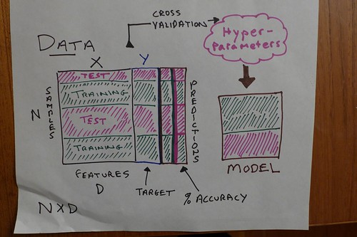
In these machine learning examples, we pick a Series Y column to be predicted, by all the other columns in DataFrame X.
The predicting is done according to a model, which creates itself by using training data, wherein the actual Y values (Survived or not) are provided.
Models come in many flavors: linear and logistical regression, random forest, neural network and more.
Once we have a model, we can test it against the training data for its predictive power, and more to the point, we can test it against testing data not yet seen by the model.
We would expect a model to be more accurate (have a higher success rate) vis-a-vis the training data it trains on, versus testing data. Even if not perfect, is our model accurate enough, even on test data, to be usable in the field?
Logistic Regression
Often used to predict a true or false outcome, based on features. Think of eligible verus ineligible for a benefit, based on features.
In contrast, linear regression, probably the simplest model, predicts a continuous range of outputs. Think of predicting a specific salary range or housing price based on features.
The curve to imagine, with logistic regression, is called a "sigmoid" and it takes on y values between two boundaries, corresponding to our yes / no logic. As with linear regression, the algorithm is geared to be multivariate.
The Python ecosystem is well endowed with machine learning and statistics packages that contain the various model types. We will turn to sci-kit learn for our needs, imported as sklearn. If you installed the Anaconda distro, it's likely already present, otherwise, you'll need to install it from the cloud.
from sklearn.model_selection import train_test_split
from sklearn.linear_model import LogisticRegression
from sklearn.metrics import accuracy_score
X = titanic_data.drop(columns = ['Survived'], axis=1)
Y = titanic_data['Survived']
Splitting into test and training data sets, after we've already "cut the cake" between X and Y, gives us a total of four data sets we need to keep track of. The training and test sets go together.
# a step along the way, almost always taken.
X_train, X_test, Y_train, Y_test = train_test_split(X,Y, test_size=0.2, random_state=2)
The Survived column is missing from X_train.
X_train
| Age | SibSp | Parch | Fare | is_group | is_alone | Sex_female | Sex_male | Embarked_C | Embarked_Q | Embarked_S | Pclass_1 | Pclass_2 | Pclass_3 | |
|---|---|---|---|---|---|---|---|---|---|---|---|---|---|---|
| 109 | 19.000 | 1 | 0 | 24.150 | 0 | 0 | True | False | False | True | False | False | False | True |
| 130 | 33.000 | 0 | 0 | 7.896 | 0 | 1 | False | True | True | False | False | False | False | True |
| 72 | 21.000 | 0 | 0 | 73.500 | 1 | 1 | False | True | False | False | True | False | True | False |
| 66 | 29.000 | 0 | 0 | 10.500 | 0 | 1 | True | False | False | False | True | False | True | False |
| 123 | 32.500 | 0 | 0 | 13.000 | 0 | 1 | True | False | False | False | True | False | True | False |
| ... | ... | ... | ... | ... | ... | ... | ... | ... | ... | ... | ... | ... | ... | ... |
| 76 | 24.000 | 0 | 0 | 7.896 | 0 | 1 | False | True | False | False | True | False | False | True |
| 43 | 3.000 | 1 | 2 | 41.579 | 0 | 0 | True | False | True | False | False | False | True | False |
| 22 | 15.000 | 0 | 0 | 8.029 | 0 | 1 | True | False | False | True | False | False | False | True |
| 73 | 26.000 | 1 | 0 | 14.454 | 0 | 0 | False | True | True | False | False | False | False | True |
| 15 | 55.000 | 0 | 0 | 16.000 | 0 | 1 | True | False | False | False | True | False | True | False |
124 rows × 14 columns
Y_train # the Survived column we want to predict
109    1
130    0
72     0
66     1
123    1
      ..
76     0
43     1
22     1
73     0
15     1
Name: Survived, Length: 124, dtype: int64
model = LogisticRegression() # the model type we plan to use
model.fit(X_train, Y_train) # a training session molds the model
LogisticRegression()In a Jupyter environment, please rerun this cell to show the HTML representation or trust the notebook.
On GitHub, the HTML representation is unable to render, please try loading this page with nbviewer.org.
LogisticRegression()
X_train_prediction = model.predict(X_train) # test it
X_train_prediction
array([1, 0, 0, 1, 1, 0, 1, 0, 0, 0, 1, 1, 0, 0, 0, 1, 0, 1, 0, 0, 0, 0,
       0, 0, 0, 0, 0, 0, 0, 0, 0, 0, 1, 1, 0, 1, 0, 0, 0, 0, 0, 0, 0, 0,
       1, 0, 0, 0, 0, 1, 1, 1, 1, 0, 0, 1, 0, 0, 0, 1, 1, 0, 0, 1, 0, 0,
       0, 0, 1, 0, 0, 0, 0, 0, 0, 0, 1, 0, 1, 1, 0, 0, 0, 0, 0, 0, 1, 1,
       0, 0, 0, 0, 1, 0, 0, 0, 0, 0, 0, 0, 0, 1, 0, 0, 0, 0, 0, 0, 0, 0,
       0, 0, 1, 0, 1, 1, 0, 0, 0, 0, 1, 1, 0, 1])
training_data_accuracy = accuracy_score(Y_train, X_train_prediction)
print('Accuracy score of training data : ', training_data_accuracy)
Accuracy score of training data : 0.8467741935483871
The expected drop-off in accuracy, given new data:
X_test_prediction = model.predict(X_test)
test_data_accuracy = accuracy_score(Y_test, X_test_prediction)
print('Accuracy score of test data : ', test_data_accuracy)
Accuracy score of test data : 0.7741935483870968
Random Forest
This well-known algorithm creates several Decision Trees, which are yes / no decision sequences aimed at classifying your samples. Think of the game of "20 questions" wherein one person thinks of an object, and the other person tries to guess it within 20 yes or no questions. "Is it bigger than a bread box?" is a typical question people use to allude to this little game.
A decision tree is a formalized series of such question. A lot of decision trees make a random forest. The many trees get to vote on each sample. Having several classifiers in the picture working together is what we call an ensemble.
from sklearn.ensemble import RandomForestClassifier
rf_model = RandomForestClassifier()
rf_model.fit(X_train, Y_train)
RandomForestClassifier()In a Jupyter environment, please rerun this cell to show the HTML representation or trust the notebook.
On GitHub, the HTML representation is unable to render, please try loading this page with nbviewer.org.
RandomForestClassifier()
X_train_prediction = rf_model.predict(X_train)
training_data_accuracy = accuracy_score(Y_train, X_train_prediction)
print('Accuracy score of training data : ', training_data_accuracy)
Accuracy score of training data : 1.0
X_test_prediction = rf_model.predict(X_test)
test_data_accuracy = accuracy_score(Y_test, X_test_prediction)
print('Accuracy score of test data : ', test_data_accuracy)
Accuracy score of test data : 0.7741935483870968
Multi-Layer Perceptron
from sklearn.neural_network import MLPClassifier
mlp_model = rf_model = MLPClassifier()
mlp_model.fit(X_train, Y_train)
MLPClassifier()In a Jupyter environment, please rerun this cell to show the HTML representation or trust the notebook.
On GitHub, the HTML representation is unable to render, please try loading this page with nbviewer.org.
MLPClassifier()
X_train_prediction = mlp_model.predict(X_train)
training_data_accuracy = accuracy_score(Y_train, X_train_prediction)
print('Accuracy score of training data : ', training_data_accuracy)
Accuracy score of training data : 0.6693548387096774
X_test_prediction = mlp_model.predict(X_test)
test_data_accuracy = accuracy_score(Y_test, X_test_prediction)
print('Accuracy score of test data : ', test_data_accuracy)
Accuracy score of test data : 0.6129032258064516
