
Change Point Detection in SAR Amplitude Time Series Data
Franz J Meyer; University of Alaska Fairbanks & Josef Kellndorfer, Earth Big Data, LLC

This notebook applies Change Point Detection on a deep multi-temporal SAR image data stack acquired by Sentinel-1. Specifically, the lab applies the method of Cumulative Sums to perform change detection on a 60 image deep Sentinel-1 data stack over Niamey, Niger.
In this notebook we introduce the following data analysis concepts:
- The concepts of time series slicing by month, year, and date.
- The concepts and workflow of Cumulative Sum-based change point detection.
- The identification of change dates for each identified change point.
Important Note about JupyterHub
Your JupyterHub server will automatically shutdown when left idle for more than 1 hour. Your notebooks will not be lost but you will have to restart their kernels and re-run them from the beginning. You will not be able to seamlessly continue running a partially run notebook.
import url_widget as url_w
notebookUrl = url_w.URLWidget()
display(notebookUrl)
from IPython.display import Markdown
from IPython.display import display

notebookUrl = notebookUrl.value
user = !echo $JUPYTERHUB_USER
env = !echo $CONDA_PREFIX
if env[0] == '':
    env[0] = 'Python 3 (base)'
if env[0] != '/home/jovyan/.local/envs/rtc_analysis':
    display(Markdown(f'<text style=color:red><strong>WARNING:</strong></text>'))
    display(Markdown(f'<text style=color:red>This notebook should be run using the "rtc_analysis" conda environment.</text>'))
    display(Markdown(f'<text style=color:red>It is currently using the "{env[0].split("/")[-1]}" environment.</text>'))
    display(Markdown(f'<text style=color:red>Select the "rtc_analysis" from the "Change Kernel" submenu of the "Kernel" menu.</text>'))
    display(Markdown(f'<text style=color:red>If the "rtc_analysis" environment is not present, use <a href="{notebookUrl.split("/user")[0]}/user/{user[0]}/notebooks/conda_environments/Create_OSL_Conda_Environments.ipynb"> Create_OSL_Conda_Environments.ipynb </a> to create it.</text>'))
    display(Markdown(f'<text style=color:red>Note that you must restart your server after creating a new environment before it is usable by notebooks.</text>'))
0. Importing Relevant Python Packages
Our first step is to import the necessary python libraries into your Jupyter Notebook:
%%capture
from pathlib import Path
from copy import deepcopy

import pandas as pd
from osgeo import gdal # for Info
gdal.UseExceptions()
import numpy as np

%matplotlib inline
import matplotlib
import matplotlib.pylab as plt
import matplotlib.patches as patches

import opensarlab_lib as asfn
asfn.jupytertheme_matplotlib_format()
1. Load Data Stack for this Lab
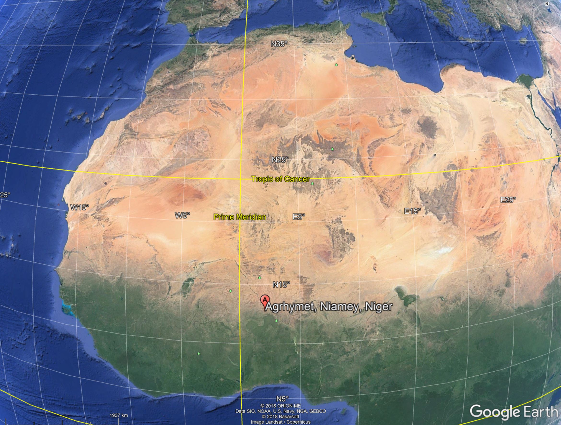
This notebook will be using a 60-image deep C-band Sentinel-1 SAR data stack over Niamey, Niger to demonstrate the concepts of time series change detection. The data are available to us through the services of the Alaska Satellite Facility.
Specifically we will use a small image segment over the campus of AGRHYMET Regional Centre, a regional organization supporting West Africa in the use or remote sensing.
This site was picked as we had information about construction going on at this site sometime in the 2015 - 2017 time frame. Land was cleared and a building was erected. In this notebook, we will see if we can detect the construction activity and if we are able to determine when construction began and when it ended.
In this case, we will retrieve the relevant data from an Amazon Web Service (AWS) cloud storage bucket.
1.1 Download The Data:
Before we download anything, create a working directory for this analysis and change into it:
path = Path("/home/jovyan/notebooks/SAR_Training/English/Master/data_Change_Detection_Amplitude_Time_Series_Example")

if not path.is_dir():
    path.mkdir()
Download the data from the AWS bucket:
!aws --region=us-west-2 --no-sign-request s3 cp s3://asf-jupyter-data-west/Niamey.zip $path/Niamey.zip
Unzip the file and clean up:
niamey_path = path/"Niamey.zip"
asfn.asf_unzip(str(path), str(niamey_path))

if niamey_path.is_file():
    niamey_path.unlink()
1.2 Switch to the Data Directory:
The following lines set variables that capture path variables needed for data processing. Change into the unzipped /cra directory and define variables for names of the files containing data and image information:
cra_path = niamey_path.cwd()/'data_Change_Detection_Amplitude_Time_Series_Example/cra'
date_file = None
image_file = None

if cra_path.exists():
    date_file = str(list(cra_path.rglob('S32631X402380Y1491460sS1_A_vv_0001_A_mtfil.dates')).pop())
    image_file = str(list(cra_path.rglob('S32631X402380Y1491460sS1_A_vv_0001_A_mtfil.vrt')).pop())
1.3 Assess Image Acquisition Dates
Before we start analyzing the available image data, we want to examine the content of our data stack. To do so, we read the image acquisition dates for all files in the time series and create a pandas date index:
with open(date_file, 'r') as d:
    dates = d.readlines()
time_index = pd.DatetimeIndex(dates)
j = 1
print('Bands and dates for', image_file)
for i in time_index:
    print("{:4d} {}".format(j, i.date()), end=' ')
    j += 1
    if j%5 == 1: print()
raster_stack = gdal.Open(image_file).ReadAsArray()
1.5 Lay the groundwork for saving plots and level-3 products.
Create a directory in which to store our output, and move into it:
product_path = path.cwd()/'data_Change_Detection_Amplitude_Time_Series_Example/plots_and_products'

if not product_path.exists():
    print(f'Created {product_path}')
    product_path.mkdir()
We will need the upper-left and lower-right corner coordinates when saving our products as GeoTiffs. In this situation, you have been given a pre-subset vrt image stack.
Retrieve the corner coordinates from the vrt using gdal.Info():
vrt = gdal.Open(image_file)
vrt_info = gdal.Info(vrt, format='json')
coords = [vrt_info['cornerCoordinates']['upperLeft'], vrt_info['cornerCoordinates']['lowerRight']]
print(coords)
Retrieve the utm zone from the vrt:
utm_zone = vrt_info['coordinateSystem']['wkt'].split(',')[-1][0:-2]
print(f"utm zone: {utm_zone}")
Write a function to convert our plots into GeoTiffs:
# do not include a file extension in out_filename
# extent must be in the form of a list: [[upper_left_x, upper_left_y], [lower_right_x, lower_right_y]]
def geotiff_from_plot(source_image, out_filename, extent, utm_zone, cmap=None, vmin=None, vmax=None, interpolation=None, dpi=300):
    plt.figure()
    plt.axis('off')
    plt.imshow(source_image, cmap=cmap, vmin=vmin, vmax=vmax, interpolation=interpolation)
    temp = Path(f"{out_filename}_temp.png")
    plt.savefig(temp, dpi=dpi, transparent='true', bbox_inches='tight', pad_inches=0)

    cmd = f"gdal_translate -of Gtiff -a_ullr {extent[0][0]} {extent[0][1]} {extent[1][0]} {extent[1][1]} -a_srs EPSG:{utm_zone} {temp} {out_filename}.tiff"
    !{cmd}
    try:
        temp.unlink()
    except FileNotFoundError:
        print('File Not Found')
        pass
2. Plot the Global Means of the Time Series
To accomplish this task, complete the following steps:
- Conversion to power-scale
- Compute mean values
- Convert to dB-scale
- Create time series of means using Pandas
- Plot time series of means
Convert to Power-scale:
caldB = -83
calPwr = np.power(10.0, caldB/10.0)
raster_stack_pwr = np.power(raster_stack, 2.0) * calPwr
Compute means:
rs_means_pwr = np.mean(raster_stack_pwr, axis=(1, 2))
Convert to dB-scale:
rs_means_dB = 10.0 * np.log10(rs_means_pwr)
Make a pandas time series object:
ts = pd.Series(rs_means_dB,index=time_index)
Use pandas to plot the time series object with band numbers as data point labels. Save the plot as a png (time_series_means.png):
plt.rcParams.update({'font.size': 14})
plt.figure(figsize=(16, 8))
plt.title(f"Time Series of Means")
ts.plot()
xl = plt.xlabel('Date')
yl = plt.ylabel('$\overline{\gamma^o}$ [dB]')
for xyb in zip(ts.index, rs_means_dB, range(1, len(ts)+1)):
    plt.annotate(xyb[2], xy=xyb[0:2])
plt.grid()

plt.savefig(f'{product_path}/time_series_means.png', dpi=72)
3. Generate Time Series for Point Locations or Subsets
In python, we can use the matrix slicing tools (similar to those used in Matlab) to obtain subsets of the data. For example, to pick one pixel at a line/pixel location and obtain all band values, use:
[:, line, pixel] notation.
Or, if we are interested in a subset at a offset location we can use:
[:, yoffset:(yoffset+yrange), xoffset:(xoffset+xrange)]
In the section below we will learn how to generate time series plots for point locations (pixels) or areas (e.g. a 5x5 window region). To show individual bands, we define a show_image function which incorporates the matrix slicing from above.
3.1 Plotting Time Series for Subset
Write a function to plot the calibrated time series for a pre-defined subset:
# Preconditions:
# raster_stack must be a stack of images in SAR power units
# time_index must be a pandas date-time index
# band_number must represent a valid bandnumber in the raster_stack
def show_image(raster_stack, time_index, band_number, output_filename=None, subset=None, vmin=None, vmax=None):
    fig = plt.figure(figsize=(16, 8))
    ax1 = fig.add_subplot(121)
    ax2 = fig.add_subplot(122)

    # If vmin or vmax are None we use percentiles as limits:
    if vmin == None:
        vmin = np.percentile(raster_stack[band_number-1].flatten(), 5)
    if vmax == None:
        vmax = np.percentile(raster_stack[band_number-1].flatten(), 95)

    ax1.imshow(raster_stack[band_number-1], cmap='gray', vmin=vmin, vmax=vmax)
    ax1.set_title(f'Image Band {band_number} {time_index[band_number-1].date()}')
    if subset == None:
        bands, ydim, xdim = raster_stack.shape
        subset = (0, 0, xdim, ydim)

    ax1.add_patch(patches.Rectangle((subset[0], subset[1]), subset[2], subset[3], fill=False, edgecolor='red'))
    ax1.xaxis.set_label_text('Pixel')
    ax1.yaxis.set_label_text('Line')
    ax1.legend(['Subset AOI'], loc='best')

    ts_pwr = np.mean(raster_stack[:, subset[1]:(subset[1]+subset[3]), subset[0]:(subset[0]+subset[2])], axis=(1,2))
    ts_dB = 10.0 * np.log10(ts_pwr)
    ax2.plot(time_index, ts_dB)
    ax2.yaxis.set_label_text('$\gamma^o$ [dB]')
    ax2.set_title('$\gamma^o$ Backscatter Time Series')
    # Add a vertical line for the date where the image is displayed
    ax2.axvline(time_index[band_number-1], color='green')
    ax2.legend(['Time Series', f'Band {band_number} Date'], loc='best')
    plt.grid()

    fig.autofmt_xdate()

    if output_filename:
        plt.savefig(f'{product_path}/{output_filename}', dpi=72)
        print(f"Saved plot: {output_filename}")
Call show_image() on different bands to compare the information content of different time steps in our area of interest.
Call show_image() on band number 24:
band_number = 24
subset = [5, 20, 3, 3]
show_image(raster_stack_pwr, time_index, band_number, subset=subset, output_filename=f"band_{band_number}.png")
Call show_image() on band number 43:
band_number = 43
show_image(raster_stack_pwr, time_index, band_number, subset=subset, output_filename=f"band_{band_number}.png")
3.2 Helper Function to Generate a Time Series Object
Write a function that creates an object representing the time series for an image subset:
# Extract the means along the time series axes
# raster shape is time steps, lines, pixels.
# With axis=1,2, we average lines and pixels for each time step (axis 0)
# returns pandas time series object
def timeSeries(raster_stack_pwr, time_index, subset, ndv=0.0):
    raster = raster_stack_pwr.copy()
    if ndv != np.nan:
        raster[np.equal(raster, ndv)] = np.nan
    ts_pwr = np.nanmean(raster[:,subset[1]:(subset[1]+subset[3]), subset[0]:(subset[0]+subset[2])], axis=(1, 2))
    # convert the means to dB
    ts_dB = 10.0 * np.log10(ts_pwr)
    # make the pandas time series object
    ts = pd.Series(ts_dB, index=time_index)
    return ts
Call timeSeries() to make a time series object for the chosen subset:
ts = timeSeries(raster_stack_pwr, time_index, subset)
Plot the time series object:
fig = ts.plot(figsize=(16, 4))
fig.yaxis.set_label_text('mean dB')
fig.set_title('Time Series for Chosen Subset')
plt.grid()
4. Create Seasonal Subsets of Time Series Records
Let's expand upon SAR time series analysis. Often it is desirable to subset time series by season or months to compare data acquired under similar weather/growth/vegetation cover conditions. For example, in analyzing C-Band backscatter data, it might be useful to limit comparative analysis to dry season observations only as soil moisture might confuse signals during the wet seasons. To subset time series along the time axis we will make use of the following Pandas datatime index tools:
- month
- day of year
Extract a hectare-sized area around our subset location (5,20,5,5):
subset = (5, 20, 5, 5)
time_series_1 = timeSeries(raster_stack_pwr, time_index, subset)
Convert the time series to a pandas DataFrame to allow for more processing options.
data_frame = pd.DataFrame(time_series_1, index=ts.index, columns=['g0'])
Label the data value column as 'g0' for $\gamma^0$ and plot the time series backscatter profile:
ylim = (-15, -5)
data_frame.plot(figsize=(16, 4))
plt.title('Sentinel-1 C-VV Time Series Backscatter Profile, Subset: 5,20,5,5  ')
plt.ylabel('$\gamma^o$ [dB]')
plt.ylim(ylim)
_ = plt.legend(["C-VV Time Series"])
plt.grid()
4.1 Change Start Date of Time Series to November 2015
Plot the cropped time series and save it as a png (time_series_backscatter_profile.png):
data_frame_sub1 = data_frame[data_frame.index>'2015-11-01']
# Plot
data_frame_sub1.plot(figsize=(16, 4))
plt.title('Sentinel-1 C-VV Time Series Backscatter Profile, Subset: {}'.format(subset))
plt.ylabel('$\gamma^o$ [dB]')
plt.ylim(ylim)
_ = plt.legend(["C-VV Time Series"])
plt.grid()
plt.savefig(f'{product_path}/time_series_backscatter_profile', dpi=72)
4.2 Subset Time Series by Months
Using the Pandas DateTimeIndex object index.month and numpy's logical_and function, we can easily subset the time series by month:
Create subset data_frames. In one, replace the data from June-February with NaNs. In the other, replace the data from March-May with NaNs:
data_frame_sub2 = deepcopy(data_frame_sub1)
for index, row in data_frame_sub2.iterrows():
    if index.month < 3 or index.month > 5:
        row['g0'] = np.nan

data_frame_sub3 = deepcopy(data_frame_sub1)
for index, row in data_frame_sub3.iterrows():
    if index.month > 2 and index.month < 6:
        row['g0'] = np.nan
Plot the time series backscatter profile for March - May. Save the plot as a png (march2may_time_series_backscatter_profile.png):
# Plot
fig, ax = plt.subplots(figsize=(16, 4))
data_frame_sub2.plot(ax=ax)
plt.title(f'Sentinel-1 C-VV Time Series Backscatter Profile, Subset: {subset}')
plt.ylabel('$\gamma^o$ [dB]')
plt.ylim(ylim)
_ = plt.legend(["C-VV Time Series (March - May)"], loc='best')
plt.grid()
plt.savefig(f'{product_path}/march2may_time_series_backscatter_profile', dpi=72)
Using numpy's invert function, we can invert a selection. In this example, we extract all other months from the time series.
Plot the time series backscatter profile for June - Feburary. Save the plot as a png (june2feb_time_series_backscatter_profile.png):
# Plot
fig, ax = plt.subplots(figsize=(16, 4))
data_frame_sub3.plot(ax=ax)
plt.title(f'Sentinel-1 C-VV Time Series Backscatter Profile, Subset: {subset}')
plt.ylabel('$\gamma^o$ [dB]')
plt.ylim(ylim)
_ = plt.legend(["C-VV Time Series (June-February)"], loc='best')
plt.grid()
plt.savefig(f'{product_path}/june2feb_time_series_backscatter_profile', dpi=72)
4.3 Split Time Series by Year to Compare Year-to-Year Patterns
Sometimes it is useful to compare year-to-year $\sigma^0$ values to identify changes in backscatter characteristics. This helps to distinguish true change from seasonal variability.
Split the time series into different years:
data_frame_by_year = data_frame_sub1.groupby(pd.Grouper(freq="YE"))
Plot the split time series. Save the plot as a png (yearly_time_series_backscatter_profile.png):
fig, ax = plt.subplots(figsize=(16, 4))
for label, df in data_frame_by_year:
    df.g0.plot(ax=ax, label=label.year)
plt.legend()
# data_frame_by_year.plot(ax=ax)
plt.title('Sentinel-1 C-VV Time Series Backscatter Profile, Subset: {}'.format(subset))
plt.ylabel('$\gamma^o$ [dB]')
plt.ylim(ylim)
plt.grid()
plt.savefig(f'{product_path}/yearly_time_series_backscatter_profile', dpi=72)
4.4 Create a Pivot Table to Group Years and Sort Data for Plotting Overlapping Time Series
Pivot Tables are a technique in data processing. They enable a person to arrange and rearrange (or "pivot") statistics in order to draw attention to useful information. To do so, we first add columns for day-of-year and year to the data frame:
# Add day of year
data_frame_sub1 = data_frame_sub1.assign(doy=data_frame_sub1.index.dayofyear)
# Add year
data_frame_sub1 = data_frame_sub1.assign(year=data_frame_sub1.index.year)
Create a pivot table which has day-of-year as the index and years as columns:
pivot_table = pd.pivot_table(data_frame_sub1, index=['doy'], columns=['year'], values=['g0'])
# Set the names for the column indices
pivot_table.columns.set_names(['g0', 'year'], inplace=True)
print(pivot_table.head(10))
print('...\n',pivot_table.tail(10))
As we can see, there are NaN values on the days in a year where no acquisition took place. Now we use time weighted interpolation to fill the dates for all the observations in any given year. For time weighted interpolation to work we need to create a dummy year as a date index, perform the interpolation, and reset the index to the day of year.
Create a dummy year as a date index:
# Add fake dates for year 100 to enable time sensitive interpolation
# of missing values in the pivot table
year_doy = ['2100-{}'.format(x) for x in pivot_table.index]
y100_doy=pd.DatetimeIndex(pd.to_datetime(year_doy,format='%Y-%j'))

# make a copy of the piv table and add two columns
pivot_table_2 = pivot_table.copy()
pivot_table_2 = pivot_table_2.assign(d100=y100_doy) # add the fake year dates
pivot_table_2 = pivot_table_2.assign(doy=pivot_table_2.index) # add doy as a column to replace as index later again

# Set the index to the dummy year
pivot_table_2.set_index('d100', inplace=True, drop=True)
Perform the time-weighted interpolation:
pivot_table_2 = pivot_table_2.interpolate(method='time')
Reset the index to the day of year:
pivot_table_2.set_index('doy', inplace=True, drop=True)
Inspect the new pivot table and see whether we interpolated the NaN values where it made sense:
print(pivot_table_2.head(10))
print('...\n',pivot_table_2.tail(10))
Plot the time series data with overlapping years. Save the plot as a png (overlapping_years_time_series_backscatter_profile.png):
pivot_table_2.plot(figsize=(16, 8))
plt.title('Sentinel-1 C-VV Time Series Backscatter Profile,\
Subset: 5,20,5,5  ')
plt.ylabel('$\gamma^o$ [dB]')
plt.xlabel('Day of Year')
_ = plt.ylim(ylim)
plt.grid()
plt.savefig(f'{product_path}/overlapping_years_time_series_backscatter_profile', dpi=72)
5. Time Series Change Detection
Now we are ready to perform efficient change detection on the time series data. We will discuss two approaches:
- Year-to-year differencing of the subsetted time series
- Cumulative Sum-based change detection
Set a dB change threshold:
threshold = 3
Calculate the difference between years (2016 and 2017):
diff_2017_2016 = pivot_table_2.g0[2017] - pivot_table_2.g0[2016]
5.1 Change Detection based on Year-to-Year Differencing
Compute and plot the differences between the interpolated time series and look for change using a threshold value. Save the plot as a png (year2year_differencing_time_series.png):
_ = diff_2017_2016.plot(kind='line', figsize=(16,8))
plt.title('Year-to-Year Difference Time Series')
plt.ylabel('$\Delta\gamma^o$ [dB]')
plt.xlabel('Day of Year')
plt.grid()
plt.savefig(f'{product_path}/year2year_differencing_time_series', dpi=72)
Calculate the days-of-year on which the threshold was exceeded:
threshold_exceeded = diff_2017_2016[abs(diff_2017_2016) > threshold]
print(threshold_exceeded)
From the threshold_exceeded dataframe we can infer the first date at which the threshold was exceeded. We would label this date as a change point. As an additional criteria for labeling a change point, one can also consider the number of observations after an identified change point that also exceeded the threshold. If only one or two observations differed from the year before this could be considered an outlier. Additional smoothing of the time series may sometimes be useful to avoid false detections.
5.2 Cumulative Sums for Change Detection
Another approach to detect change in regularly acquired data is employing the method of cumulative sums. Changes are determined by comparing the time series data against its mean. A full explanation and examples from the financial sector can be found at http://www.variation.com/cpa/tech/changepoint.html
5.2.A First let's consider a time series and its mean observation:
We look at two full years of observations from Sentinel-1 data for an area where we suspect change. In the following, we define $X$ as our time series
\begin{equation} X = (X_1,X_2,...,X_n) \end{equation}with $X_i$ being the SAR backscatter values at times $i=1,...,n$ and $n$ is the number of observations in the time series.
Create a times series of the subset and calculate the backscatter values:
subset = (5, 20, 3, 3)
time_series_1 = timeSeries(raster_stack_pwr, time_index, subset)
backscatter_values = time_series_1[time_series_1.index>'2015-10-31']
5.2.B Filtering the time series for outliers:
It is advantageous in noisy SAR time series like those from C-Band Sentinel-1 data to reduce noise by applying a filter along the time axis. Pandas offers a "rolling" function for these purposes. Using the rolling function, we will apply a median filter to our data.
Calculate the median backscatter values and plot them against the original values. Save the plot as a png (Original vs. Median Time Series):
backscatter_values_median = backscatter_values.rolling(5, center=True).median()
fig, ax = plt.subplots(figsize=(16, 4))
backscatter_values_median.plot()
backscatter_values.plot()
plt.title('Original vs. Median Time Series')
plt.ylabel('$\gamma^o$ [dB]')
plt.xlabel('Time')
plt.grid()
plt.savefig(f'{product_path}/original_vs_median_time_series', dpi=72)
Calculate the time series' mean value and plot it against the original values. Save the plot as a png (original_time_series_vs_mean_val.png):
fig, ax = plt.subplots(figsize=(16, 4))
backscatter_values.plot()
plt.title('Original Time Series vs. Mean Value')
plt.ylabel('$\gamma^o$ [dB]')
ax.axhline(backscatter_values.mean(), color='red')
_ = plt.legend(['$\gamma^o$', '$\overline{\gamma^o}$'])
plt.grid()
plt.savefig(f'{product_path}/original_time_series_vs_mean_val', dpi=72)
Calculate the time series' mean value and plot it against the median values. Save the plot as a png (median_time_series_vs_mean_val.png):
backscatter_values_mean = backscatter_values.mean()

fig, ax = plt.subplots(figsize=(16, 4))
backscatter_values_median.plot()
plt.title('Median Time Series vs. Mean Value')
plt.ylabel('$\gamma^o$ [dB]')
ax.axhline(backscatter_values.mean(), color='red')
_ = plt.legend(['$\gamma^o$', '$\overline{\gamma^o}$'])
plt.grid()
plt.savefig(f'{product_path}/median_time_series_vs_mean_val', dpi=72)
5.2.C Calculate the Residuals of the Time Series Against the Mean $\overline{\gamma^o}$:
To get to the residual, we calculate
\begin{equation} R = X_i - \overline{X} \end{equation}Calculate the residuals:
residuals = backscatter_values - backscatter_values_mean
5.2.D Calculate Cumulative Sum of the Residuals: The cumulative sum is defined as:
\begin{equation} S = \displaystyle\sum_1^n{R_i} \end{equation}Calculate and plot the cumulative sum of the residuals. Save the plot as a png (cumulative_sum_residuals.png):
sums = residuals.cumsum()

_ = sums.plot(figsize=(16, 6))
plt.title('Cumulative Sum of the Residuals')
plt.ylabel('Cummulative Sum $S$ [dB]')
plt.xlabel('Time')
plt.grid()
plt.savefig(f'{product_path}/cumulative_sum_residuals', dpi=72)
The cumulative sum is a good indicator of change in the time series. An estimator for the magnitude of change is given as the difference between the maximum and minimum value of the cumulative sum $S$:
\begin{equation} S_{DIFF} = S_{MAX} - S_{MIN} \end{equation}Calculate the magnitude of change:
change_mag = sums.max() - sums.min()
print('Change magnitude: %5.3f dB' % (change_mag))
5.2.E Identify Change Point in the Time Series: A candidate change point is identified from $S$ at the time where $S_{MAX}$ is found:
\begin{equation} T_{{CP}_{before}} = T(S_i = S_{MAX}) \end{equation}with $T_{{CP}_{before}}$ being the timestamp of the last observation before the identified change point, $S_i$ is the cumulative sum of $R$ with $i=1,...n$, and $n$ is the number of observations in the time series.
The first observation after a change occurred ($T_{{CP}_{after}}$) is then found as the first observation in the time series following $T_{{CP}_{before}}$.
Calculate $T_{{CP}_{before}}$:
change_point_before = sums[sums==sums.max()].index[0]
print('Last date before change occurred: {}'.format(change_point_before.date()))
Calculate $T_{{CP}_{after}}$:
change_point_after = sums[sums.index > change_point_before].index[0]
print('First date after change occurred: {}'.format(change_point_after.date()))
5.2.F Determine our Confidence in the Identified Change Point using Bootstrapping: We can determine if an identified change point is indeed a valid detection by randomly reordering the time series and comparing the various $S$ curves. During this "bootstrapping" approach, we count how many times the $S_{DIFF}$ values are greater than $S_{{DIFF}_{random}}$ of the identified change point.
After bootstrapping, we define the confidence level $CL$ in a detected change point according to:
\begin{equation} CL = \frac{N_{GT}}{N_{bootstraps}} \end{equation}where $N_{GT}$ is the number of times $S_{DIFF}$ > $S_{{DIFF}_{random}}$ and $N_{bootstraps}$ is the number of bootstraps randomizing $R$.
As another quality metric we can also calculate the significance $CP_{significance}$ of a change point according to:
\begin{equation} CP_{significance} = 1 - \left( \frac{\sum_{b=1}^{N_{bootstraps}}{S_{{DIFF}_{{random}_i}}}}{N_{bootstraps}} \middle/ S_{DIFF} \right) \end{equation}The closer $CP_{significance}$ is to 1, the more significant the change point.
Write a function that implements the bootstrapping algorithm:
# pyplot must be imported as plt
import random
def bootstrap(n_bootstraps, name, sums, residuals, output_file=False):
    fig, ax = plt.subplots(figsize=(16,6))
    ax.set_ylabel('Cumulative Sums of the Residuals')
    change_mag_random_sum = 0
    change_mag_random_max = 0 # to keep track of the maximum change magnitude of the bootstrapped sample
    qty_change_mag_above_random = 0 # to keep track of the maximum Sdiff of the bootstrapped sample
    print("Running Bootstrapping for %4.1f iterations ..." % (n_bootstraps))
    colors = ['C0', 'C1', 'C2', 'C3', 'C4', 'C5', 'C6', 'C7', 'C8', 'C9', 'c', 'm', 'y', 'k', 'g']
    for i in range(n_bootstraps):
        r_random = residuals.sample(frac=1)  # Randomize the time steps of the residuals
        residuals_random = pd.Series(r_random.values, index=residuals.index)

        sums_random = residuals_random.cumsum()
        change_mag_random = sums_random.max() - sums_random.min()
        change_mag_random_sum += change_mag_random
        if change_mag_random > change_mag_random_max:
            change_mag_random_max = change_mag_random
        if change_mag > change_mag_random:
            qty_change_mag_above_random += 1

        sums_random.plot(ax=ax, color=random.choice(colors), label='_nolegend_')

        if ((i+1)/n_bootstraps*100) % 10 == 0:
            print("\r%4.1f percent completed ..." % ((i+1)/n_bootstraps*100), end='\r', flush=True)
    sums.plot(ax=ax, color='r', linewidth=3)
    fig.legend(['S Curve for Candidate Change Point'])
    print(f"Bootstrapping Complete")
    _ = ax.axhline(change_mag_random_sum/n_bootstraps, color='b')
    plt.grid()
    if output_file:
        plt.savefig(f"{product_path}/bootstrap_{name}_{n_bootstraps}", dpi=72)
        print(f"Saved plot: bootstrap_{name}_{n_bootstraps}.png")
    return [qty_change_mag_above_random, change_mag_random_sum]
n_bootstraps = 2000
bootstrapped_change_mag = bootstrap(n_bootstraps, "", sums, residuals, output_file=True)
Call the bootstrap function with a sample size of 2000:
Based on the bootstrapping results, we can now calculate Confidence Level $CL$ and Significance $CP_{significance}$ for our candidate change point.
Calculate the confidence level:
confidence_level = 1.0 * bootstrapped_change_mag[0] / n_bootstraps
print('Confidence Level for change point {} percent'.format(confidence_level*100.0))
Calculate the change point significance:
change_point_significance = 1.0 - (bootstrapped_change_mag[1]/n_bootstraps)/change_mag
print('Change point significance metric: {}'.format(change_point_significance))
5.2.G TRICK: Detrending of Time Series Before Change Detection to Improve Robustness:
De-trending the time series with global image means improves the robustness of change point detection as global image time series anomalies stemming from calibration or seasonal trends are removed prior to time series analysis. This de-trending needs to be performed with large subsets so real change is not influencing the image statistics.
NOTE: Due to the small size of our subset, we will see some distortions when we detrend the time series.
Let's start by building a global image means time series and plot the global means. Save the plot as a png (global_means_time_series.png):
means_pwr = np.mean(raster_stack_pwr, axis=(1, 2))
means_dB = 10.0 * np.log10(means_pwr)
global_means_ts = pd.Series(means_dB, index=time_index)
global_means_ts = global_means_ts[global_means_ts.index > '2015-10-31'] # filter dates
global_means_ts = global_means_ts.rolling(5, center=True).median()
global_means_ts.plot(figsize=(16, 6))
plt.title('Time Series of Global Means')
plt.ylabel('[dB]')
plt.xlabel('Time')
plt.grid()
plt.savefig(f"{product_path}/global_means_time_series", dpi=72)
Compare the time series of global means (above) to the time series of our small subset (below):
backscatter_values.plot(figsize=(16, 6))
plt.title('Sentinel-1 C-VV Time Series Backscatter Profile,\
Subset: 5,20,5,5  ')
plt.ylabel('[dB]')
plt.xlabel('Time')
plt.grid()
There are some signatures of the global seasonal trend in our subset time series. To remove these signatures and get a cleaner time series of change, we subtract the global mean time series from our subset time series.
De-trend the subset and re-plot the backscatter profile. Save the plot (detrended_time_series.png):
backscatter_minus_seasonal = backscatter_values - global_means_ts
backscatter_minus_seasonal.plot(figsize=(16, 6))
plt.title('De-trended Sentinel-1 C-VV Time Series Backscatter Profile, Subset: 5,20,5,5')
plt.ylabel('[dB]')
plt.xlabel('Time')
plt.grid()
plt.savefig(f"{product_path}/detrended_time_series", dpi=72)
Save a plot comparing the original, global means, and detrended time-series (globalMeans_original_detrended_time_series.png):
means_pwr = np.mean(raster_stack_pwr, axis=(1, 2))
means_dB = 10.0 * np.log10(means_pwr)
global_means_ts = pd.Series(means_dB, index=time_index)
global_means_ts = global_means_ts[global_means_ts.index > '2015-10-31'] # filter dates
global_means_ts = global_means_ts.rolling(5, center=True).median()
global_means_ts.plot(figsize=(16, 6))
backscatter_values.plot(figsize=(16, 6))
backscatter_minus_seasonal = (backscatter_values - global_means_ts)
backscatter_minus_seasonal.plot(figsize=(16, 6))
plt.title('Time Series of Global Means')
plt.ylabel('[dB]')
plt.xlabel('Time')
plt.legend(['Global Means TS', 'Backscatter', 'Detrended Backscatter'], loc='best')
plt.grid()
plt.savefig(f"{product_path}/globalMeans_original_detrended_time_series", dpi=72)
Recalculate and plot the residuals based on the de-trended data:
residuals = backscatter_minus_seasonal - backscatter_values_mean
Compute, plot, and save the cumulative sum of the detrended time series (cumualtive_sum_detrended_time_series.png):
sums = residuals.cumsum()
_ = sums.plot(figsize=(16, 6))
plt.title("Cumulative Sum of the Detrended Time Series")
plt.ylabel('CumSum $S$ [dB]')
plt.xlabel('Time')
plt.grid()
plt.savefig(f"{product_path}/cumualtive_sum_detrended_time_series", dpi=72)
Detect Change Point and extract related change dates:
detrended_change_point_before = sums[sums==sums.max()].index[0]
print('Last date before change occurred: {}'.format(detrended_change_point_before.date()))

detrended_change_point_after = sums[sums.index > detrended_change_point_before].index[0]
print('First date after change occurred: {}'.format(detrended_change_point_after.date()))
Perform bootstrapping:
n_bootstraps = 2000
bootstrapped_change_mag = bootstrap(n_bootstraps, "detrended", sums, residuals, output_file=True)
Calculate the confidence level:
detrended_confidence_level = bootstrapped_change_mag[0] / n_bootstraps
print('Confidence Level for change point {} percent'.format(confidence_level*100.0))
Note how the change point significance $CP_{significance}$ has increased in the detrended time series:
detrended_change_point_significance = 1.0 - (bootstrapped_change_mag[1]/n_bootstraps) / change_mag
print('Change point significance metric: {}'.format(change_point_significance))
6. Cumulative Sum-based Change Detection Across an Entire Image
With numpy arrays we can apply the concept of cumulative sum change detection analysis effectively on the entire image stack. We take advantage of array slicing and axis-based computing in numpy. Axis 0 is the time domain in our raster stacks.
6.1 We first create our time series stack:
Filter out the first layer (Keep Dates >= '2015-11-17'):
raster_stack = raster_stack_pwr
raster_stack_sub = raster_stack_pwr[1:, :, :]
time_index_sub = time_index[1:]
Run the following code cell if you wish to change to dB scale:
raster_stack = 10.0 * np.log10(raster_stack_sub)
Plot and save Band-1 (band_1.png):
plt.figure(figsize=(12, 8))
band_number = 0
vmin = np.percentile(raster_stack[band_number], 5)
vmax = np.percentile(raster_stack[band_number], 95)
plt.title('Band  {} {}'.format(band_number+1, time_index_sub[band_number].date()))
plt.imshow(raster_stack[0], cmap='gray', vmin=vmin, vmax=vmax)
_ = plt.colorbar()
plt.savefig(f'{product_path}/band_1.png', dpi=300, transparent='true')
Save the plot as a GeoTiff (band_1.tiff):
%%capture
geotiff_from_plot(raster_stack[0], f'{product_path}/band_1', coords, utm_zone, cmap='gray', dpi=600)
6.2 Calculate Mean Across Time Series to Prepare for Calculation of Cumulative Sum $S$:
Plot and save the the raster stack mean (raster_stack_mean.png):
raster_stack_mean = np.mean(raster_stack, axis=0)
plt.figure(figsize=(12, 8))
plt.imshow(raster_stack_mean, cmap='gray')
_ = plt.colorbar()
plt.savefig(f'{product_path}/raster_stack_mean.png', dpi=300, transparent='true')
Save the raster stack mean as a GeoTiff (raster_stack_mean.tiff):
%%capture
geotiff_from_plot(raster_stack_mean, f'{product_path}/raster_stack_mean', coords, utm_zone, cmap='gray', dpi=600)
Calculate the residuals:
residuals = raster_stack - raster_stack_mean
Close img, as it is no longer needed in the notebook:
radar_stack = None
Plot and save the residuals for band 1 (residuals_band_1.png):
plt.figure(figsize=(12, 8))
plt.imshow(residuals[0])
plt.title('Residuals for Band  {} {}'.format(band_number+1, time_index_sub[band_number].date()))
_ = plt.colorbar()
plt.savefig(f'{product_path}/residuals_band_1', dpi=300, transparent='true')
Save the residuals for band 1 as a GeoTiff (residuals_band_1.tiff):
%%capture
geotiff_from_plot(residuals[0], f'{product_path}/residuals_band_1', coords, utm_zone, dpi=600)
6.3 Calculate Cumulative Sum $S$ as well as Change Magnitude $S_{diff}$:
Plot and save the cumulative sum max, min, and change magnitude (Smax_Smin_Sdiff.png):
sums = np.cumsum(residuals, axis=0)
sums_max = np.max(sums, axis=0)
sums_min = np.min(sums, axis=0)
change_mag = sums_max - sums_min
fig, ax = plt.subplots(1, 3, figsize=(16, 4))
vmin = sums_min.min()
vmax = sums_max.max()
sums_max_plot = ax[0].imshow(sums_max, vmin=vmin, vmax=vmax)
ax[0].set_title('$S_{max}$')
ax[1].imshow(sums_min, vmin=vmin, vmax=vmax)
ax[1].set_title('$S_{min}$')
ax[2].imshow(change_mag, vmin=vmin, vmax=vmax)
ax[2].set_title('Change Magnitude')
fig.subplots_adjust(right=0.8)
cbar_ax = fig.add_axes([0.85, 0.15, 0.02, 0.7])
_ = fig.colorbar(sums_max_plot, cax=cbar_ax)
plt.savefig(f'{product_path}/Smax_Smin_Sdiff', dpi=300, transparent='true')
Save Smax as a GeoTiff (Smax.tiff):
%%capture
geotiff_from_plot(sums_max, f'{product_path}/Smax', coords, utm_zone, vmin=vmin, vmax=vmax)
Save Smin as a GeoTiff (Smin.tiff):
%%capture
geotiff_from_plot(sums_min, f'{product_path}/Smin', coords, utm_zone, vmin=vmin, vmax=vmax)
Save the change magnitude as a GeoTiff (Sdiff.tiff):
%%capture
geotiff_from_plot(change_mag, f'{product_path}/Sdiff', coords, utm_zone, vmin=vmin, vmax=vmax)
6.4 Mask $S_{diff}$ With a-priori Threshold To Idenfity Change Candidate Pixels:
To identified change candidate pixels, we can threshold $S_{diff}$ to reduce computation of the bootstrapping. For land cover change we would not expect more than 5-10% change pixels in a landscape. So, if the test region is reasonably large, setting a threshold for expected change to 10% is appropriate. In our example we'll start out with a very conservative threshold of 20%.
Plot and save the histogram for the change magnitude and the change magnitude cumulative distribution function (Sdiff_histogram_CDF.png):
plt.rcParams.update({'font.size': 14})
fig = plt.figure(figsize=(14, 6)) # Initialize figure with a size
ax1 = fig.add_subplot(121)  # 121 determines: 2 rows, 2 plots, first plot
ax2 = fig.add_subplot(122)
# Second plot: Histogram
# IMPORTANT: To get a histogram, we first need to *flatten*
# the two-dimensional image into a one-dimensional vector.
histogram = ax1.hist(change_mag.flatten(), bins=200, range=(0, np.max(change_mag)))
ax1.xaxis.set_label_text('Change Magnitude')
ax1.set_title('Change Magnitude Histogram')
plt.grid()
n, bins, patches = ax2.hist(change_mag.flatten(), bins=200, range=(0, np.max(change_mag)), cumulative='True', density='True', histtype='step', label='Empirical')
ax2.xaxis.set_label_text('Change Magnitude')
ax2.set_title('Change Magnitude CDF')
plt.grid()
plt.savefig(f'{product_path}/Sdiff_histogram_CDF', dpi=72, transparent='true')
Using this threshold, we can create a plot to visualize our change candidate areas. Save the plot (change_candidate.png):
precentile = 0.8
out_indicies = np.where(n>precentile)
threshold_indicies = np.min(out_indicies)
threshold = bins[threshold_indicies]
print('At the {}% percentile, the threshold value is {:2.2f}'.format(precentile*100,threshold))

change_mag_mask = change_mag < threshold
plt.figure(figsize=(12, 8))
plt.title('Change Candidate Areas (black)')
_ = plt.imshow(change_mag_mask, cmap='gray')
plt.savefig(f'{product_path}/change_candidate', dpi=300, transparent='true')
Save the change candidate plot as a GeoTiff (change_candidate.tiff):
%%capture
geotiff_from_plot(change_mag_mask, f'{product_path}/change_candidate', coords, utm_zone, cmap='gray')
6.5 Bootstrapping to Prepare for Change Point Selection:
We can now perform bootstrapping over the candidate pixels. The workflow is as follows:
- Filter our residuals to the change candidate pixels
- Perform bootstrapping over candidate pixels
Mask the residuals in pixels below the change point threshold
residuals_mask = np.broadcast_to(change_mag_mask, residuals.shape)
residuals_masked = np.ma.array(residuals, mask=residuals_mask)
Using the masked residuals, re-compute the cumulative sums:
sums_masked = np.ma.cumsum(residuals_masked, axis=0)
Plot the min sums, max sums, and change magnitude of the masked subset (masked_Smax_Smin_Sdiff.png):
sums_masked_max = np.ma.max(sums_masked, axis=0)
sums_masked_min = np.ma.min(sums_masked, axis=0)
change_mag = sums_masked_max - sums_masked_min
fig, ax = plt.subplots(1, 3, figsize=(16, 4))
vmin = sums_masked_min.min()
vmax = sums_masked_max.max()
sums_masked_max_plot = ax[0].imshow(sums_masked_max, vmin=vmin, vmax=vmax)
ax[0].set_title('$S_{max}$')
ax[1].imshow(sums_masked_min, vmin=vmin, vmax=vmax)
ax[1].set_title('$S_{min}$')
ax[2].imshow(change_mag, vmin=vmin, vmax=vmax)
ax[2].set_title('Change Magnitude')
fig.subplots_adjust(right=0.8)
cbar_ax = fig.add_axes([0.85, 0.15, 0.02, 0.7])
_ = fig.colorbar(sums_masked_max_plot, cax=cbar_ax)
plt.savefig(f'{product_path}/masked_Smax_Smin_Sdiff', dpi=300, transparent='true')
Save the Smax of the masked subset as a GeoTiff (masked_Smax.tiff):
%%capture
geotiff_from_plot(sums_masked_max, f'{product_path}/masked_Smax', coords, utm_zone, vmin=vmin, vmax=vmax)
Save the Smin of the masked subset as a GeoTiff (masked_Smin.tiff):
%%capture
geotiff_from_plot(sums_masked_min, f'{product_path}/masked_Smin', coords, utm_zone, vmin=vmin, vmax=vmax)
Save the change magnitude of the masked subset as a GeoTiff (masked_Sdiff.tiff):
%%capture
geotiff_from_plot(change_mag, f'{product_path}/masked_Sdiff', coords, utm_zone, vmin=vmin, vmax=vmax)
Perform bootstrapping:
random_index = np.random.permutation(residuals_masked.shape[0])
residuals_random = residuals_masked[random_index,:,:]
n_bootstraps = 2000  # bootstrap sample size
# to keep track of the maxium Sdiff of the bootstrapped sample:
change_mag_random_max = np.ma.copy(change_mag)
change_mag_random_max[~change_mag_random_max.mask] = 0
# to compute the Sdiff sums of the bootstrapped sample:
change_mag_random_sum = np.ma.copy(change_mag)
change_mag_random_sum[~change_mag_random_max.mask] = 0
# to keep track of the count of the bootstrapped sample
qty_change_mag_above_random = change_mag_random_sum
qty_change_mag_above_random[~qty_change_mag_above_random.mask] = 0
print("Running Bootstrapping for %4.1f iterations ..." % (n_bootstraps))
for i in range(n_bootstraps):
    # For efficiency, we shuffle the time axis index and use that
    #to randomize the masked array
    random_index = np.random.permutation(residuals_masked.shape[0])
    # Randomize the time step of the residuals
    residuals_random = residuals_masked[random_index, :, :]
    sums_random = np.ma.cumsum(residuals_random, axis=0)
    sums_random_max = np.ma.max(sums_random, axis=0)
    sums_random_min = np.ma.min(sums_random, axis=0)
    change_mag_random = sums_random_max - sums_random_min
    change_mag_random_sum += change_mag_random
    change_mag_random_max[np.ma.greater(change_mag_random, change_mag_random_max)] = \
    change_mag_random[np.ma.greater(change_mag_random, change_mag_random_max)]
    qty_change_mag_above_random[np.ma.greater(change_mag, change_mag_random)] += 1
    if ((i+1)/n_bootstraps*100)%10 == 0:
        print("\r%4.1f percent completed ..." % ((i+1)/n_bootstraps*100), end='\r', flush=True)
print(f"Bootstrapping Complete.      ")
6.6 Extract Confidence Metrics and Select Final Change Points:
We first compute for all pixels the confidence level $CL$, the change point significance metric $CP_{significance}$ and the product of the two as our confidence metric for identified change points. Plot and save them (confidence_change_point.png):
confidence_level = qty_change_mag_above_random / n_bootstraps
change_point_significance = 1.0 - (change_mag_random_sum/n_bootstraps) / change_mag
#Plot
fig, ax = plt.subplots(1, 3 ,figsize=(16, 4))
a = ax[0].imshow(confidence_level*100)
fig.colorbar(a, ax=ax[0])
ax[0].set_title('Confidence Level %')
a = ax[1].imshow(change_point_significance)
fig.colorbar(a, ax=ax[1])
ax[1].set_title('Change Point Significance')
a = ax[2].imshow(confidence_level*change_point_significance)
fig.colorbar(a, ax=ax[2])
_ = ax[2].set_title('Confidence Level\nx\nChange Point Significance')
plt.savefig(f'{product_path}/confidence_change_point', dpi=300, transparent='true')
Save the confidence level of the masked subset as a GeoTiff (confidence_level.tiff):
%%capture
geotiff_from_plot(confidence_level*100, f'{product_path}/confidence_level', coords, utm_zone)
Save the change point significance of the masked subset as a GeoTiff (change_point.tiff):
%%capture
geotiff_from_plot(change_point_significance, f'{product_path}/change_point', coords, utm_zone)
Save the confidence level x change point significance of the masked subset as a GeoTiff (CL_x_CP.tiff):
%%capture
geotiff_from_plot(confidence_level*change_point_significance, f'{product_path}/CL_x_CP', coords, utm_zone)
Set a change point threshold of 5:
change_point_threshold = 5
Create and save a plot showing the final change points (change_point_thresh.png):
fig = plt.figure(figsize=(12, 8))
ax = fig.add_subplot(1, 1, 1)
plt.title('Detected Change Pixels based on Threshold %2.1f' % (change_point_threshold))
a = ax.imshow(confidence_level*change_point_significance < change_point_threshold, cmap='cool')
plt.savefig(f'{product_path}/change_point_thresh', dpi=300, transparent='true')
Save the thresholded change point significance of the masked subset as a GeoTiff (change_point_thresh.tiff):
%%capture
geotiff_from_plot(confidence_level*change_point_significance < change_point_threshold,
                  f'{product_path}/change_point_thresh', coords, utm_zone, cmap='cool')
6.7 Derive Timing of Change for Each Change Pixel:
Our last step in the identification of the change points is to extract the timing of the change. We will produce a raster layer that shows the band number of the first date after a change was detected. We will make use of the numpy indexing scheme.
Create a combined mask of the first threshold and the identified change points after the bootstrapping:
# make a mask of our change points from the new threhold and the previous mask
change_point_mask = np.ma.mask_or(confidence_level*change_point_significance<change_point_threshold,
                                  confidence_level.mask)
# Broadcast the mask to the shape of the masked S curves
change_point_mask2 = np.broadcast_to(change_point_mask, sums_masked.shape)
# Make a numpy masked array with this mask
change_point_raster = np.ma.array(sums_masked.data, mask=change_point_mask2)
To retrieve the dates of the change points we find the band indices in the time series along the time axis where the maximum of the cumulative sums was located. Numpy offers the "argmax" function for this purpose.
change_point_index = np.ma.argmax(np.abs(change_point_raster), axis=0)
change_indices = list(np.unique(change_point_index))
change_indices.remove(0)
print(f"Change Indicies:\n{change_indices}")
# Look up the dates from the indices to get the change dates
all_dates = time_index[time_index>'2015-10-31']
change_dates = [str(all_dates[x].date()) for x in change_indices]
print(f"\nChange Dates:\n{change_dates}")
Plot the change dates using the change point index raster and save it as a png (change_dates.png):
ticks = change_indices
tick_labels = change_dates

cmap = matplotlib.colormaps.get_cmap('tab20')
fig, ax = plt.subplots(figsize=(12, 12))
cax = ax.imshow(change_point_index, interpolation='nearest', cmap=cmap)

ax.set_title('Dates of Change')
cbar = fig.colorbar(cax, ticks=ticks, orientation='horizontal')
_ = cbar.ax.set_xticklabels(tick_labels, size=10, rotation=45, ha='right')
plt.savefig(f'{product_path}/change_dates', dpi=300, transparent='true')
Save the Dates of Change plot as a GeoTiff (change_dates.tiff):
Note: The GeoTiff does not include a colorbar. Date/color correlations can be identified in change_dates.png.
%%capture
geotiff_from_plot(change_point_index, f'{product_path}/change_dates', coords, utm_zone, interpolation='nearest', cmap=cmap)
Change_Detection_Amplitude_Time_Series_Example.ipynb - Version 1.5.1 - February 2024
Version Changes
- Adjust how we create the residuals_random Pandas.Series in the bootstrapping function to support Pandas updates
- Use matplotlib.colormaps.get_cmap