![]()

0. Introduction
Python in the Scientific environment
Principal Python Packages for scientific purposes
Anaconda & conda

http://conda.pydata.org/docs/intro.html
Conda is a package manager application that quickly installs, runs, and updates packages and their dependencies. The conda command is the primary interface for managing installations of various packages. It can query and search the package index and current installation, create new environments, and install and update packages into existing conda environments.
from IPython.display import HTML
HTML('<iframe src="http://conda.pydata.org/docs/_downloads/conda-cheatsheet.pdf" width="700" height="400"></iframe>')
Main objectives of this workshop
- Provide you with a first insight into the principal Python tools & libraries used in Science:
- conda.
- Jupyter Notebook.
- NumPy, matplotlib, SciPy
- Provide you with the basic skills to face basic tasks such as:
- Show other common libraries:
- Pandas, scikit-learn (some talks & workshops will focus on these packages)
- SymPy
- Numba ¿?
1. Jupyter Notebook
![]()
The Jupyter Notebook is a web application that allows you to create and share documents that contain live code, equations, visualizations and explanatory text. Uses include: data cleaning and transformation, numerical simulation, statistical modeling, machine learning and much more.
It has been widely recognised as a great way to distribute scientific papers, because of the capability to have an integrated format with text and executable code, highly reproducible. Top level investigators around the world are already using it, like the team behind the Gravitational Waves discovery (LIGO), whose analysis was translated to an interactive dowloadable Jupyter notebook. You can see it here: https://github.com/minrk/ligo-binder/blob/master/GW150914_tutorial.ipynb
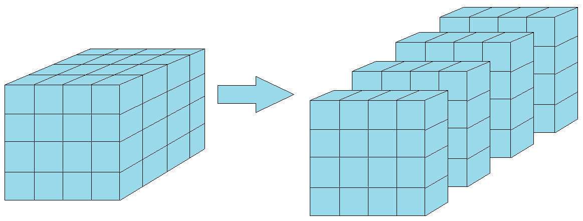
2. Using arrays: NumPy

ndarray object
| index | 0 | 1 | 2 | 3 | ... | n-1 | n |
|---|---|---|---|---|---|---|---|
| value | 2.1 | 3.6 | 7.8 | 1.5 | ... | 5.4 | 6.3 |
- N-dimensional data structure.
- Homogeneously typed.
- Efficient!
A universal function (or ufunc for short) is a function that operates on ndarrays. It is a “vectorized function".
# importing numpy
# performance list sum
1000 loops, best of 3: 1.54 ms per loop
# performance array sum

%timeit np.sum(array)
10000 loops, best of 3: 97.8 µs per loop
Array creation
one_dim_array =
array([1, 2, 3, 4])
two_dim_array =
array([[1, 2, 3],
       [4, 5, 6],
       [7, 8, 9]])
# size & shape
9
(3, 3)
# data type
dtype('int64')
# usual arrays
array([ 0, 1, 2, 3, 4, 5, 6, 7, 8, 9, 10, 11, 12, 13, 14])
# changing the shape
array([[ 0,  1,  2,  3,  4],
       [ 5,  6,  7,  8,  9],
       [10, 11, 12, 13, 14]])
# linspace
array([  0. ,   0.5,   1. ,   1.5,   2. ,   2.5,   3. ,   3.5,   4. ,
         4.5,   5. ,   5.5,   6. ,   6.5,   7. ,   7.5,   8. ,   8.5,
         9. ,   9.5,  10. ])
Basic slicing
one_dim_array
1
two_dim_array
9
[start:stop:step]
array([ 0,  2,  4,  6,  8, 10, 12, 14, 16, 18, 20, 22, 24, 26, 28, 30, 32,
       34, 36, 38, 40, 42, 44, 46, 48, 50, 52, 54, 56, 58, 60, 62, 64, 66,
       68, 70, 72, 74, 76, 78, 80, 82, 84, 86, 88, 90, 92, 94, 96, 98])
# Chess board
chess_board = np.zeros([8, 8], dtype=int)
# your code

chess_board
array([[0, 1, 0, 1, 0, 1, 0, 1],
       [1, 0, 1, 0, 1, 0, 1, 0],
       [0, 1, 0, 1, 0, 1, 0, 1],
       [1, 0, 1, 0, 1, 0, 1, 0],
       [0, 1, 0, 1, 0, 1, 0, 1],
       [1, 0, 1, 0, 1, 0, 1, 0],
       [0, 1, 0, 1, 0, 1, 0, 1],
       [1, 0, 1, 0, 1, 0, 1, 0]])
2. Drawing: Matplotlib

# drawing the chessboard
<matplotlib.image.AxesImage at 0x7f1aad09df98>

Operations & linalg
# numpy functions
x =
y =
# plotting
[<matplotlib.lines.Line2D at 0x7f1aacb554e0>]

# another function
[<matplotlib.lines.Line2D at 0x7f1aacabbdd8>]

# transpose
two_dim_array =
array([[10, 40, 77],
       [25, 25, 68],
       [33, 16, 91]])
# matrix multiplication
array([[ 3641,  3119,  3733],
       [ 2632,  2713,  3176],
       [10497,  9813, 11910]])
# matrix vector
array([ 240.4, 250.8, 783.1])
# inv
array([[-0.05372256,  0.00140303,  0.01923512],
       [ 0.10898393,  0.07381761, -0.05250057],
       [-0.03598099, -0.05634759,  0.03394433]])
# eigenvectors & eigenvalues
(array([ 133.6946629,  -17.266221 ,    9.5715581]),
 array([[-0.29580975, -0.74274264,  0.0661375 ],
        [-0.24477775,  0.65983255, -0.79576005],
        [-0.92335283,  0.1138173 ,  0.60198985]]))
Air quality data
from IPython.display import HTML
HTML('<iframe src="http://www.mambiente.munimadrid.es/sica/scripts/index.php" \
            width="700" height="400"></iframe>')
Loading the data
# Linux command
!head ./data/barrio_del_pilar-20160322.csv

# Windows
# !gc log.txt | select -first 10 # head
Estación: Barrio del Pilar;;;;
Fecha;Hora;CO;NO2;O3
;;mg/m³;µg/m³;µg/m³
22/03/2016;01:00;0.2;14;73
22/03/2016;02:00;0.2;10;77
22/03/2016;03:00;0.2;9;75
22/03/2016;04:00;0.2;3;81
22/03/2016;05:00;0.2;3;81
22/03/2016;06:00;0.2;6;79
22/03/2016;07:00;0.2;24;59
# loading the data
# ./data/barrio_del_pilar-20160322.csv
data2016 =
array([[   0.2,   14. ,   73. ],
       [   0.2,   10. ,   77. ],
       [   0.2,    9. ,   75. ],
       [   0.2,    3. ,   81. ],
       [   0.2,    3. ,   81. ],
       [   0.2,    6. ,   79. ],
       [   0.2,   24. ,   59. ],
       [   0.3,   48. ,   37. ],
       [   0.3,   40. ,   43. ],
       [   0.3,   41. ,   44. ],
       [   0.3,   20. ,   68. ],
       [   0.3,   17. ,   74. ],
       [   0.2,   14. ,   84. ],
       [   0.3,   16. ,   88. ],
       [   0.3,   15. ,   94. ],
       [   0.4,   29. ,   81. ],
       [   0.3,   23. ,   82. ],
       [   0.3,   26. ,   81. ],
       [   0.3,   30. ,   75. ],
       [   0.4,   57. ,   39. ],
       [   0.4,   73. ,   17. ],
       [   0.4,   51. ,   42. ],
       [   0.4,   72. ,   16. ],
       [   0.4,   61. ,   28. ],
       [   0.3,   25. ,   62. ],
       [   0.3,   21. ,   64. ],
       [   0.3,   40. ,   39. ],
       [   0.4,   52. ,   19. ],
       [   0.4,   47. ,    8. ],
       [   0.4,   42. ,    8. ],
       [   0.5,   68. ,    8. ],
       [   0.6,   71. ,    9. ],
       [   0.9,   76. ,   10. ],
       [   0.7,   63. ,   29. ],
       [   0.3,   27. ,   66. ],
       [   0.3,   13. ,   88. ],
       [   0.2,   10. ,   92. ],
       [   0.3,   10. ,   98. ],
       [   0.3,   11. ,   99. ],
       [   0.3,   12. ,   99. ],
       [   0.2,   11. ,   98. ],
       [   0.2,    8. ,  101. ],
       [   0.2,   13. ,   92. ],
       [   0.2,   23. ,   79. ],
       [   0.5,   40. ,   56. ],
       [   0.6,   49. ,   43. ],
       [   0.5,   66. ,   25. ],
       [   0.4,   47. ,   44. ],
       [   0.3,   18. ,   76. ],
       [   0.3,   25. ,   64. ],
       [   0.3,   16. ,   77. ],
       [   0.3,   16. ,   59. ],
       [   0.3,   34. ,   31. ],
       [   0.3,   27. ,   33. ],
       [   0.3,   44. ,   17. ],
       [   0.4,   45. ,    9. ],
       [   0.5,   52. ,   22. ],
       [   0.4,   37. ,   53. ],
       [   0.3,   21. ,   73. ],
       [   0.3,   20. ,   76. ],
       [   0.3,   24. ,   76. ],
       [   0.4,   38. ,   71. ],
       [   0.3,   32. ,   78. ],
       [   0.3,   21. ,   89. ],
       [   0.2,   10. ,  105. ],
       [   0.3,   15. ,  102. ],
       [   0.3,   21. ,   93. ],
       [   0.3,   45. ,   63. ],
       [   0.4,   59. ,   47. ],
       [   0.4,   59. ,   44. ],
       [   0.7,   99. ,    9. ],
       [   0.6,   88. ,    9. ],
       [   0.8,   93. ,    9. ],
       [   0.9,   89. ,    9. ],
       [   0.8,   84. ,    8. ],
       [   0.5,   64. ,   10. ],
       [   0.4,   58. ,   11. ],
       [   0.5,   53. ,    9. ],
       [   0.4,   41. ,    8. ],
       [   0.5,   43. ,    9. ],
       [   0.5,   45. ,   13. ],
       [   0.6,   51. ,   25. ],
       [   0.5,   44. ,   40. ],
       [   0.4,   36. ,   59. ],
       [   0.4,   36. ,   68. ],
       [   0.3,   26. ,   84. ],
       [   0.3,   16. ,   98. ],
       [   0.3,   17. ,   97. ],
       [   0.3,   24. ,   89. ],
       [   0.3,   17. ,   99. ],
       [   0.3,   12. ,  100. ],
       [   0.3,   42. ,   61. ],
       [   0.4,   52. ,   44. ],
       [   0.5,   54. ,   39. ],
       [   0.5,   60. ,   28. ],
       [   0.6,   73. ,   13. ],
       [   0.5,   58. ,   23. ],
       [   0.4,   58. ,   16. ],
       [   0.5,   61. ,   10. ],
       [   0.5,   59. ,    9. ],
       [   0.4,   50. ,    9. ],
       [   0.3,   31. ,   10. ],
       [   0.4,   36. ,    9. ],
       [   0.6,   45. ,    9. ],
       [   0.5,   43. ,   18. ],
       [   0.5,   37. ,   24. ],
       [   0.5,   40. ,   38. ],
       [   0.4,   26. ,   59. ],
       [   0.3,   14. ,   67. ],
       [   0.3,   12. ,   64. ],
       [   0.3,   13. ,   62. ],
       [   0.2,   10. ,   63. ],
       [   0.2,    7. ,   58. ],
       [   0.2,    8. ,   53. ],
       [   0.2,   11. ,   51. ],
       [   0.3,   16. ,   47. ],
       [   0.2,   19. ,   42. ],
       [   0.3,   22. ,   38. ],
       [   0.3,   23. ,   36. ],
       [   0.3,   16. ,   43. ],
       [   0.2,    9. ,   49. ],
       [   0.2,    6. ,   48. ],
       [   nan,    nan,    nan],
       [   0.2,    4. ,   64. ],
       [   0.2,    3. ,   89. ],
       [   0.2,    4. ,   90. ],
       [   0.2,    3. ,   92. ],
       [   0.2,    6. ,   89. ],
       [   0.3,   11. ,   83. ],
       [   0.3,    9. ,   87. ],
       [   0.3,    8. ,   84. ],
       [   0.3,   10. ,   82. ],
       [   0.3,   10. ,   80. ],
       [   0.3,   12. ,   80. ],
       [   0.3,   12. ,   81. ],
       [   0.3,    8. ,   84. ],
       [   0.3,   10. ,   85. ],
       [   0.2,   10. ,   85. ],
       [   0.2,   14. ,   82. ],
       [   0.3,   18. ,   72. ],
       [   0.3,   28. ,   60. ],
       [   0.3,   30. ,   55. ],
       [   0.3,   21. ,   61. ],
       [   0.3,   16. ,   63. ],
       [   0.3,   12. ,   65. ],
       [   0.2,    9. ,   67. ],
       [   0.2,    5. ,   70. ],
       [   0.2,    5. ,   69. ],
       [   0.2,    6. ,   65. ],
       [   0.2,    7. ,   63. ],
       [   0.3,   16. ,   55. ],
       [   0.3,   30. ,   45. ],
       [   0.3,   38. ,   39. ],
       [   0.3,   37. ,   41. ],
       [   0.3,   29. ,   53. ],
       [   0.3,   27. ,   53. ],
       [   0.3,   27. ,   49. ],
       [   0.3,   23. ,   54. ],
       [   0.3,   22. ,   57. ],
       [   0.3,   19. ,   61. ],
       [   0.3,   17. ,   63. ],
       [   0.3,   22. ,   59. ],
       [   0.3,   27. ,   53. ],
       [   0.3,   29. ,   50. ],
       [   0.3,   34. ,   44. ],
       [   0.3,   33. ,   45. ],
       [   0.3,   26. ,   50. ],
       [   0.3,   19. ,   56. ],
       [   0.2,   11. ,   63. ],
       [   0.2,    8. ,   63. ],
       [   0.2,    9. ,   58. ],
       [   0.2,    6. ,   63. ],
       [   0.2,    5. ,   66. ],
       [   0.2,    7. ,   62. ],
       [   0.3,   18. ,   53. ],
       [   0.4,   38. ,   37. ],
       [   0.4,   49. ,   28. ],
       [   0.4,   45. ,   35. ],
       [   0.3,   34. ,   47. ],
       [   0.3,   24. ,   62. ],
       [   0.3,   24. ,   68. ],
       [   0.3,   28. ,   68. ],
       [   0.3,   23. ,   78. ],
       [   0.3,   21. ,   82. ],
       [   0.3,   17. ,   87. ],
       [   0.3,   23. ,   80. ],
       [   0.3,   28. ,   75. ],
       [   0.3,   29. ,   71. ],
       [   0.3,   46. ,   50. ],
       [   0.4,   66. ,   27. ],
       [   0.3,   51. ,   38. ],
       [   0.3,   42. ,   46. ]])
Dealing with missing values
# mean
array([ nan, nan, nan])
array([ 0.33717277, 29.79581152, 55.47643979])
# masking invalid data
masked_array(data = [0.3371727748691094 29.79581151832461 55.47643979057592],
             mask = [False False False],
       fill_value = 1e+20)
data2015 =
Plotting the data
** Maximum values ** from: http://www.mambiente.munimadrid.es/opencms/export/sites/default/calaire/Anexos/valores_limite_1.pdf
- NO2
- Media anual: 40 µg/m3
- Media horaria: 200 µg/m3
(0, 220)

from IPython.display import HTML
HTML('<iframe src="http://ccaa.elpais.com/ccaa/2015/12/24/madrid/1450960217_181674.html" width="700" height="400"></iframe>')
- CO
- Máxima diaria de las medias móviles octohorarias: 10 mg/m³
# http://docs.scipy.org/doc/numpy-1.10.0/reference/generated/numpy.convolve.html
def moving_average(x, N=8):
    return np.convolve(x, np.ones(N)/N, mode='same')
<matplotlib.legend.Legend at 0x7f1aac190518>

- O3
- Máxima diaria de las medias móviles octohorarias: 120 µg/m3
- Umbral de información. 180 µg/m3
- Media horaria. Umbral de alerta. 240 µg/m3
<matplotlib.legend.Legend at 0x7f1aac0fd588>

4. Scientific functions: SciPy
![]()
scipy.linalg: ATLAS LAPACK and BLAS libraries

scipy.stats: distributions, statistical functions...

scipy.integrate: integration of functions and ODEs

scipy.optimization: local and global optimization, fitting, root finding...

scipy.interpolate: interpolation, splines...

scipy.fftpack: Fourier trasnforms

scipy.signal, scipy.special, scipy.io
Temperature data
Now, we will use some temperature data from the Spanish Ministry of Agriculture.
HTML('<iframe src="http://eportal.magrama.gob.es/websiar/Ficha.aspx?IdProvincia=28&IdEstacion=1" width="700" height="400"></iframe>')
The file contains data from 2004 to 2015 (included). Each row corresponds to a day of the year, so evey 365 lines contain data from a whole year*
Note1: 29th February has been removed for leap-years. Note2: Missing values have been replaced with the immediately prior valid data.
These kind of events are better handled with Pandas!
!head data/M01_Center_Finca_temperature_data_2004_2015.csv
# mean; max; min
3.49;10.87;-2.75
5.10;10.88;-2.36
8.77;11.86;3.80
6.07;14.77;-1.36
2.48;12.06;-3.68
1.69;11.47;-3.81
2.57;9.29;-3.81
6.28;11.08;0.49
11.66;16.24;8.76
# Loading the data
temp_data =
# Importing SciPy stats
# Applying some functions: describe, mode, mean...
DescribeResult(nobs=4380, minmax=(array([ -4.21, -0.04, -11.88]), array([ 30.59, 42. , 21.77])), mean=array([ 14.03399543, 21.22098858, 6.86335388]), variance=array([ 59.25648501, 76.46548678, 44.03205308]), skewness=array([ 0.07277802, 0.10781561, -0.0989195 ]), kurtosis=array([-1.09612434, -1.11634177, -0.94371617]))
ModeResult(mode=array([[ 21. , 24.77, 0. ]]), count=array([[10, 11, 53]]))
array([ 14.03399543, 21.22098858, 6.86335388])
array([ 13.52, 20.62, 7.09])
We can also get information about percentiles!
array([ 7.65 , 13.665, 1.32 ])
1.1415525114155249
0.022831050228310501
19.315068493150687
Rearranging the data
temp_data2 = np.zeros([365, 3, 12])
# Calculating mean of mean temp

# max of max

# min of min
Let's visualize data!
Using matplotlib styles http://matplotlib.org/users/whats_new.html#styles
plt.style.available
['seaborn-deep',
 'seaborn-ticks',
 'dark_background',
 'grayscale',
 'seaborn-muted',
 'ggplot',
 'seaborn-talk',
 'seaborn-paper',
 'seaborn-poster',
 'seaborn-bright',
 'seaborn-whitegrid',
 'classic',
 'fivethirtyeight',
 'seaborn-pastel',
 'bmh',
 'seaborn-white',
 'seaborn-darkgrid',
 'seaborn-dark',
 'seaborn-colorblind',
 'seaborn-notebook',
 'seaborn-dark-palette']
# plotting max_max, min_min, mean_mean
(1, 365)

Let's see if 2015 was a normal year...
# mean vs mean_mean
(1, 365)

# and max, min 2015
But the power of Matplotlib does not end here!
For example, lets represent a function over a 2D domain!
For this we will use the contour function, which requires some special inputs...
#we will use numpy functions in order to work with numpy arrays
def funcion(x,y):
    return
# 0D: works!
funcion(3,5)
-1.9489167712635838
# 1D: works!
x = np.
plt.plot( , )
[<matplotlib.lines.Line2D at 0x7f1aa5a44f60>]

In oder to plot the 2D function, we will need a grid.
For 1D domain, we just needed one 1D array containning the X position and another 1D array containing the value.
Now, we will create a grid, a distribution of points covering a surface. For the 2D domain, we will need:
- One 2D array containing the X coordinate of the points.
- One 2D array containing the Y coordinate of the points.
- One 2D array containing the function value at the points.
The three matrices must have the exact same dimensions, because each cell of them represents a particular point.
#We can create the X and Y matrices by hand, or use a function designed to make ir easy:

#we create two 1D arrays of the desired lengths:
x_1d = np.linspace(0, 5, 5)
y_1d = np.linspace(-2, 4, 7)
#And we use the meshgrid function to create the X and Y matrices!
X, Y =
X
array([[ 0.  ,  1.25,  2.5 ,  3.75,  5.  ],
       [ 0.  ,  1.25,  2.5 ,  3.75,  5.  ],
       [ 0.  ,  1.25,  2.5 ,  3.75,  5.  ],
       [ 0.  ,  1.25,  2.5 ,  3.75,  5.  ],
       [ 0.  ,  1.25,  2.5 ,  3.75,  5.  ],
       [ 0.  ,  1.25,  2.5 ,  3.75,  5.  ],
       [ 0.  ,  1.25,  2.5 ,  3.75,  5.  ]])
Y
array([[-2., -2., -2., -2., -2.],
       [-1., -1., -1., -1., -1.],
       [ 0.,  0.,  0.,  0.,  0.],
       [ 1.,  1.,  1.,  1.,  1.],
       [ 2.,  2.,  2.,  2.,  2.],
       [ 3.,  3.,  3.,  3.,  3.],
       [ 4.,  4.,  4.,  4.,  4.]])
Note that with the meshgrid function we can only create rectangular grids
#Using Numpy arrays, calculating the function value at the points is easy!
Z
#Let's plot it!
<matplotlib.colorbar.Colorbar at 0x7f1aa5988a90>

We can try a little more resolution...
x_1d = np.???(0, 5, 100)
y_1d = np.???(-2, 4, 100)
X, Y = np.???( , )
Z = funcion(X,Y)
plt.contour(X, Y, Z)
plt.colorbar()
<matplotlib.colorbar.Colorbar at 0x7f1aa58a2278>

The countourf function is simmilar, but it colours also between the lines. In both functions, we can manually adjust the number of lines/zones we want to differentiate on the plot.
plt.contourf( , , , ,cmap=plt.cm.Spectral) #With cmap, a color map is specified
plt.colorbar()
<matplotlib.colorbar.Colorbar at 0x7f1aa5b6a978>

plt.contourf( , , , ,cmap=plt.cm.Spectral)
plt.colorbar()
<matplotlib.colorbar.Colorbar at 0x7f1aa5775c18>

#We can even combine them!
plt.contourf(X, Y, Z, np.linspace(-2, 2, 100),cmap=plt.cm.Spectral)
plt.colorbar()
cs = plt.???(X, Y, Z, np.linspace(-2, 2, 9), colors='k')
plt.clabel(cs)
<a list of 13 text.Text objects>

These functions can be enormously useful when you want to visualize something.
And remember!
Always visualize data!
Let's try it with Real data!
time_vector = np. ('data/ligo_tiempos.txt')
frequency_vector =  np. ('data/ligo_frecuencias.txt')
intensity_matrix =  np. ('data/ligo_datos.txt')
The time and frequency vectors contain the values at which the instrument was reading, and the intensity matrix, the postprocessed strength measured for each frequency at each time.
We need again to create the 2D arrays of coordinates.
time_2D, freq_2D = np.
plt. ( ) #We can manually adjust the sice of the picture
plt. ( , , ,np.linspace(0, 0.02313, 200),cmap='bone')
plt.xlabel('time (s)')
plt.ylabel('Frequency (Hz)')
plt.colorbar()
<matplotlib.colorbar.Colorbar at 0x7f1aa426e160>

Wow! What is that? Let's zoom into it!
plt.figure(figsize=(10,6))
plt.contourf(time_2D, freq_2D,intensity_matrix,np.linspace(0, 0.02313, 200),cmap = plt.cm.Spectral)
plt.colorbar()
plt.contour(time_2D, freq_2D,intensity_matrix,np.linspace(0, 0.02313, 9), colors='k')
plt.xlabel('time (s)')
plt.ylabel('Frequency (Hz)')

plt.axis([9.9, 10.05, 0, 300])
[9.9, 10.05, 0, 300]

IPython Widgets
The IPython Widgets are interactive tools to use in the notebook. They are fun and very useful to quickly understand how different parameters affect a certain function.
This is based on a section of the PyConEs 14 talk by Kiko Correoso "Hacking the notebook": http://nbviewer.jupyter.org/github/kikocorreoso/PyConES14_talk-Hacking_the_Notebook/blob/master/notebooks/Using%20Interact.ipynb
from ipywidgets import interact
#Lets define a extremely simple function:
def ejemplo(x):
    print(x)
#Try changing the value of x to True, 'Hello' or ['hello', 'world']
10
<function __main__.ejemplo>
#We can control the slider values with more precission:
9.0
<function __main__.ejemplo>
If you want a dropdown menu that passes non-string values to the Python function, you can pass a dictionary. The keys in the dictionary are used for the names in the dropdown menu UI and the values are the arguments that are passed to the underlying Python function.
10
<function __main__.ejemplo>
Let's have some fun! We talked before about frequencys and waves. Have you ever learn about AM and FM modulation? It's the process used to send radio communications!
x = np.linspace(-1, 7, 1000)

fig = plt.figure()
fig.tight_layout()

plt.subplot(211)#This allows us to display multiple sub-plots, and where to put them
plt.plot(x, np.sin(x))
plt.grid(False)
plt.title("Audio signal: modulator")

plt.subplot(212)
plt.plot(x, np.sin(50 * x))
plt.grid(False)
plt.title("Radio signal: carrier")
<matplotlib.text.Text at 0x7f1a9f67e470>

#Am modulation simply works like this:
am_wave = np.sin(50 * x) * (0.5 + 0.5 * np.sin(x))
plt.plot(x, am_wave)
[<matplotlib.lines.Line2D at 0x7f1a9f5ab4e0>]

In order to interact with it, we will need to transform it into a function
def am_mod (f_carr=50, f_mod=1, depth=0.5): #The default values will be the starting points of the sliders
interact(am_mod,
        f_carr = (1,100,2),
        f_mod = (0.2, 2, 0.1),
        depth = (0, 1, 0.1))
<function __main__.am_mod>

Other options...
5. Other packages
Symbolic calculations with SymPy

SymPy is a Python package for symbolic math. We will not cover it in depth, but let's take a picure of the basics!
# Importación
from sympy import init_session

init_session(use_latex='matplotlib') #We must start calling this function
IPython console for SymPy 1.0 (Python 3.5.1-64-bit) (ground types: python)

These commands were executed:
>>> from __future__ import division
>>> from sympy import *
>>> x, y, z, t = symbols('x y z t')
>>> k, m, n = symbols('k m n', integer=True)
>>> f, g, h = symbols('f g h', cls=Function)
>>> init_printing()

Documentation can be found at http://docs.sympy.org/1.0/
The basic unit of this package is the symbol. A simbol object has name and graphic representation, which can be different:
coef_traccion =

w =
W =
w, W
By default, SymPy takes symbols as complex numbers. That can lead to unexpected results in front of certain operations, like logarithms. We can explicitly signal that a symbol is real when we create it. We can also create several symbols at a time.
x, y, z, t = symbols('x y z t', real=True)
x.assumptions0
Expressions can be created from symbols:
expr =
expr
#We can substitute pieces of the expression:
expr.
#We can particularize on a certain value:
(sin(x) + 3 * x).
#We can evaluate the numerical value with a certain precission:
(sin(x) + 3 * x).
We can manipulate the expression in several ways. For example:
expr1 = (x ** 3 + 3 * y + 2) ** 2
expr1
expr1.
We can derivate and integrate:
expr = cos(2*x)
expr.
expr_xy = y ** 3 * sin(x) ** 2 + x ** 2 * cos(y)
expr_xy
int2 = 1 / sin(x)
x, a = symbols('x a', real=True)

int3 = 1 / (x**2 + a**2)**2
We also have ecuations and differential ecuations:
a, x, t, C = symbols('a, x, t, C', real=True)
ecuacion =
ecuacion
x = symbols('x')
f = Function('y')
ecuacion_dif =
ecuacion_dif
Data Analysis with pandas
![]()
Pandas is a package that focus on data structures and data analysis tools. We will not cover it because the next workshop, by Kiko Correoso, will develop it in depth.
Machine Learning with scikit-learn
![]()
Scikit-learn is a very complete Python package focusing on machin learning, and data mining and analysis. We will not cover it in depth because it will be the focus of many more talks at the PyData.
A world of possibilities...

Thanks for yor attention!
![]()
Any Questions?
# Notebook style
from IPython.core.display import HTML
css_file = './static/style.css'
HTML(open(css_file, "r").read())