Kinematics of particle
Marcos Duarte, Renato Naville Watanabe
Laboratory of Biomechanics and Motor Control
Federal University of ABC, Brazil
Contents
Python setup
import numpy as np
import matplotlib.pyplot as plt
%matplotlib inline
import seaborn as sns
sns.set_context("notebook", font_scale=1.2, rc={"lines.linewidth": 2, "lines.markersize": 10})
Biomechanics & Mechanics
A good knowledge of Mechanics is a necessary condition, although not sufficient!, to master Biomechanics
For this reason, we will review principles of Classical Mechanics in the context of Biomechanics.
The book Introduction to Statics and Dynamics , written by Andy Ruina and Rudra Pratap, is an excellent reference (a rigorous and yet didactic presentation of Mechanics for undergraduate students) on Classical Mechanics and we will use this book as the main reference on Mechanics and Mathematics for this brief review. The preface and first chapter of the book are a good read on how someone should study Mechanics. You should read them!
As we argued in the notebook Biomechanics, we will start with a branch of Classical Mechanics that is simpler to measure its related quantities on biological systems, the Kinematics.
There are some relevant cases in the study of human movement where modeling the human body or one of its segments as a particle might be all we need to explore the phenomenon. The concept of kinematics of a particle, for instance, can be applied to study the performance in the 100-m race; to describe spatial and temporal characteristics of a movement pattern, and to conjecture about how voluntary movements are planned (the minimum jerk hypothesis).
Now, let's review the concept of kinematics of a particle and later apply to the study of human movement.
Kinematics
Kinematics is the branch of Classical Mechanics that describes the motion of objects without consideration of the causes of motion (Wikipedia).
Kinematics of a particle is the description of the motion when the object is considered a particle.
A particle as a physical object does not exist in nature; it is a simplification to understand the motion of a body or it is a conceptual definition such as the center of mass of a system of objects.
Vectors in Kinematics
Some mechanical quantities in Kinematics (position and its derivatives) are represented as vectors and others, such as time and distance, are scalars.
A vector in Mechanics is a physical quantity with magnitude, direction, and satisfies some elementary vector arithmetic, whereas a scalar is a physical quantity that is fully expressed by a magnitude (a number) only.
For a review about scalars and vectors, see chapter 1 of Ruina and Rudra's book.
For how to use Python to work with scalars and vectors, see the notebook Scalar and Vector.
Position
Consider a point in the three-dimensional Euclidean space described in a Cartesian coordinate system (see the notebook Frame of reference for an introduction on coordinate systems in Mechanics and Biomechanics):

The position of this point in space can be represented as a triple of values each representing the coordinate at each axis of the Cartesian coordinate system following the $ \mathbf{X, Y, Z} $ convention order (which is omitted):
\begin{equation} (x,\, y,\, z) \label{eq_xyz} \end{equation}The position of a particle in space can also be represented by a vector in the Cartesian coordinate system, with the origin of the vector at the origin of the coordinate system and the tip of the vector at the point position:
\begin{equation} \overrightarrow{\mathbf{r}}(t) = x\,\hat{\mathbf{i}} + y\,\hat{\mathbf{j}} + z\,\hat{\mathbf{k}} \label{eq_rxyz} \end{equation}Where $\hat{\mathbf{i}},\, \hat{\mathbf{j}},\, \hat{\mathbf{k}}\,$ are unit vectors in the directions of the axes $ \mathbf{X, Y, Z} $.
For a review on vectors, see the notebook Scalar and vector.
With this new notation, the coordinates of a point representing the position of a particle that vary with time would be expressed by the following position vector $\overrightarrow{\mathbf{r}}(t)$:
\begin{equation} \overrightarrow{\mathbf{r}}(t) = x(t)\,\hat{\mathbf{i}} + y(t)\,\hat{\mathbf{j}} + z(t)\,\hat{\mathbf{k}} \label{eq_rxyzijk} \end{equation}A vector can also be represented in matrix form:
\begin{equation} \overrightarrow{\mathbf{r}}(t) = \begin{bmatrix} x(t) \\y(t) \\z(t) \end{bmatrix} \label{eq_rxyzmatrix} \end{equation}And the unit vectors in each Cartesian coordinate in matrix form are given by:
\begin{equation} \hat{\mathbf{i}} = \begin{bmatrix}1\\0\\0 \end{bmatrix},\; \hat{\mathbf{j}} = \begin{bmatrix}0\\1\\0 \end{bmatrix},\; \hat{\mathbf{k}} = \begin{bmatrix} 0 \\ 0 \\ 1 \end{bmatrix} \label{eq_ijk} \end{equation}Basis
In linear algebra, a set of unit linearly independent vectors as the three vectors above (orthogonal in the Euclidean space) that can represent any vector via linear combination is called a basis. A basis is the foundation of creating a reference frame and we will study how to do that other time.
Displacement
The shortest distance between two positions of a particle.
As the difference between two vectors, displacement is also a vector quantity.
\begin{equation} \mathbf{\overrightarrow{d}} = \mathbf{\overrightarrow{r}_2} - \mathbf{\overrightarrow{r}_1} \label{eq_distance} \end{equation}
Velocity
Velocity is the rate (with respect to time) of change of the position of a particle.
The average velocity between two instants is:
\begin{equation} \overrightarrow{\mathbf{v}}(t) = \frac{\overrightarrow{\mathbf{r}}(t_2)-\overrightarrow{\mathbf{r}}(t_1)}{t_2-t_1} = \frac{\Delta \overrightarrow{\mathbf{r}}}{\Delta t} \label{eq_velocity} \end{equation}The instantaneous velocity of the particle is obtained when $\Delta t$ approaches to zero, which from calculus is the first-order derivative of the position vector:
\begin{equation} \overrightarrow{\mathbf{v}}(t) = \lim_{\Delta t \to 0} \frac{\Delta \overrightarrow{\mathbf{r}}}{\Delta t} = \lim_{\Delta t \to 0} \frac{\overrightarrow{\mathbf{r}}(t+\Delta t)-\overrightarrow{\mathbf{r}}(t)}{\Delta t} = \frac{\mathrm{d}\overrightarrow{\mathbf{r}}}{dt} \label{eq_velocityderiv} \end{equation}For the movement of a particle described with respect to an inertial Frame of reference, the derivative of a vector is obtained by differentiating each vector component of the Cartesian coordinates (since the base versors $\hat{\mathbf{i}}, \hat{\mathbf{j}}, \hat{\mathbf{k}}$ are constant):
\begin{equation} \overrightarrow{\mathbf{v}}(t) = \frac{\mathrm{d}\overrightarrow{\mathbf{r}}(t)}{dt} = \frac{\mathrm{d}x(t)}{\mathrm{d}t}\hat{\mathbf{i}} + \frac{\mathrm{d}y(t)}{\mathrm{d}t}\hat{\mathbf{j}} + \frac{\mathrm{d}z(t)}{\mathrm{d}t}\hat{\mathbf{k}} \label{eq_velocityderiv2} \end{equation}Or in matrix form (and using the Newton's notation for differentiation):
\begin{equation} \overrightarrow{\mathbf{v}}(t) = \begin{bmatrix} \dot x(t) \\ \dot y(t) \\ \dot z(t) \end{bmatrix} \label{eq_velocityderiv3} \end{equation}Acceleration
Acceleration is the rate (with respect to time) of change of the velocity of a particle, which can also be given by the second-order rate of change of the position.
The average acceleration between two instants is:
\begin{equation} \overrightarrow{\mathbf{a}}(t) = \frac{\overrightarrow{\mathbf{v}}(t_2)-\overrightarrow{\mathbf{v}}(t_1)}{t_2-t_1} = \frac{\Delta \overrightarrow{\mathbf{v}}}{\Delta t} \label{eq_acc} \end{equation}Likewise, instantaneous acceleration is the first-order derivative of the velocity or the second-order derivative of the position vector:
\begin{equation} \overrightarrow{\mathbf{a}}(t) = \frac{\mathrm{d}\overrightarrow{\mathbf{v}}(t)}{\mathrm{d}t} = \frac{\mathrm{d}^2\overrightarrow{\mathbf{r}}(t)}{\mathrm{d}t^2} = \frac{\mathrm{d}^2x(t)}{\mathrm{d}t^2}\hat{\mathbf{i}} + \frac{\mathrm{d}^2y(t)}{\mathrm{d}t^2}\hat{\mathbf{j}} + \frac{\mathrm{d}^2z(t)}{\mathrm{d}t^2}\hat{\mathbf{k}} \label{eq_accderiv} \end{equation}And in matrix form:
\begin{equation} \mathbf{a}(t) = \begin{bmatrix} \ddot x(t) \\ \ddot y(t) \\ \ddot z(t) \end{bmatrix} \label{eq_accderiv2} \end{equation}For curiosity, see Notation for differentiation on the origin of the different notations for differentiation.
When the base versors change in time, for instance when the basis is attached to a rotating frame or reference, the components of the vector’s derivative is not the derivatives of its components; we will also have to consider the derivative of the basis with respect to time.
The antiderivative
As the acceleration is the derivative of the velocity which is the derivative of position, the inverse mathematical operation is the antiderivative (or integral):
\begin{equation} \begin{array}{l l} \mathbf{r}(t) = \mathbf{r}_0 + \int \mathbf{v}(t) \:\mathrm{d}t \\ \mathbf{v}(t) = \mathbf{v}_0 + \int \mathbf{a}(t) \:\mathrm{d}t \end{array} \label{eq_antiderivative} \end{equation}This part of the kinematics is presented in chapter 12, pages 605-620, of the Ruina and Rudra's book.
Some cases of motion of a particle
To deduce some trivial cases of motion of a particle (at rest, at constant speed, and at constant acceleration), we can start from the equation for its position and differentiate it to obtain expressions for the velocity and acceleration or the inverse approach, start with the equation for acceleration, and then integrate it to obtain the velocity and position of the particle. Both approachs are valid in Mechanics. For the present case, it probaly makes more sense to start with the expression for acceleration.
Particle at rest
\begin{equation} \begin{array}{l l} \overrightarrow{\mathbf{a}}(t) = 0 \\ \overrightarrow{\mathbf{v}}(t) = 0 \\ \overrightarrow{\mathbf{r}}(t) = \overrightarrow{\mathbf{r}}_0 \end{array} \label{eq_rest} \end{equation}Particle at constant speed
\begin{equation} \begin{array}{l l} \overrightarrow{\mathbf{a}}(t) = 0 \\ \overrightarrow{\mathbf{v}}(t) = \overrightarrow{\mathbf{v}}_0 \\ \overrightarrow{\mathbf{r}}(t) = \overrightarrow{\mathbf{r}}_0 + \overrightarrow{\mathbf{v}}_0t \end{array} \label{eq_constantspeed} \end{equation}Particle at constant acceleration
\begin{equation} \begin{array}{l l} \overrightarrow{\mathbf{a}}(t) = \overrightarrow{\mathbf{a}}_0 \\ \overrightarrow{\mathbf{v}}(t) = \overrightarrow{\mathbf{v}}_0 + \overrightarrow{\mathbf{a}}_0t \\ \overrightarrow{\mathbf{r}}(t) = \overrightarrow{\mathbf{r}}_0 + \overrightarrow{\mathbf{v}}_0t + \frac{1}{2}\overrightarrow{\mathbf{a}}_0 t^2 \end{array} \label{eq_constantacceleration} \end{equation}Visual representation of these cases
t = np.arange(0, 2.0, 0.02)
r0 = 1; v0 = 2; a0 = 4

plt.rc('axes',  labelsize=14,  titlesize=14)
plt.rc('xtick', labelsize=10)
plt.rc('ytick', labelsize=10)
f, axarr = plt.subplots(3, 3, sharex = True, sharey = True, figsize=(14,7))
plt.suptitle('Scalar kinematics of a particle', fontsize=20);

tones = np.ones(np.size(t))

axarr[0, 0].set_title('at rest', fontsize=14);
axarr[0, 0].plot(t, r0*tones, 'g', linewidth=4, label='$r(t)=1$')
axarr[1, 0].plot(t,  0*tones, 'b', linewidth=4, label='$v(t)=0$')
axarr[2, 0].plot(t,  0*tones, 'r', linewidth=4, label='$a(t)=0$')
axarr[0, 0].set_ylabel('r(t) [m]')
axarr[1, 0].set_ylabel('v(t) [m/s]')
axarr[2, 0].set_ylabel('a(t) [m/s$^2$]')

axarr[0, 1].set_title('at constant speed');
axarr[0, 1].plot(t, r0*tones+v0*t, 'g', linewidth=4, label='$r(t)=1+2t$')
axarr[1, 1].plot(t, v0*tones,      'b', linewidth=4, label='$v(t)=2$')
axarr[2, 1].plot(t,  0*tones,      'r', linewidth=4, label='$a(t)=0$')

axarr[0, 2].set_title('at constant acceleration');
axarr[0, 2].plot(t, r0*tones+v0*t+1/2.*a0*t**2,'g', linewidth=4,
                 label='$r(t)=1+2t+\\frac{1}{2}4t^2$')
axarr[1, 2].plot(t, v0*tones+a0*t,             'b', linewidth=4,
                 label='$v(t)=2+4t$')
axarr[2, 2].plot(t, a0*tones,                  'r', linewidth=4,
                 label='$a(t)=4$')

for i in range(3):
    axarr[2, i].set_xlabel('Time [s]');
    for j in range(3):
        axarr[i,j].set_ylim((-.2, 10))
        axarr[i,j].legend(loc = 'upper left', frameon=True, framealpha = 0.9, fontsize=14)

plt.subplots_adjust(hspace=0.09, wspace=0.07)

from sympy import Symbol, integrate, init_printing
init_printing(use_latex='mathjax')

t = Symbol('t', real=True, positive=True)
g = Symbol('g', real=True, positive=True)
v0 = Symbol('v0', real=True, positive=True, constant = True)
r0 = Symbol('r0', real=True, positive=True, constant = True)
v = integrate(g, t) + v0  # a constant has to be added
v
r = integrate(v, t) + r0  # a constant has to be added
r
Kinematics of human movement
Kinematics of the 100-m race
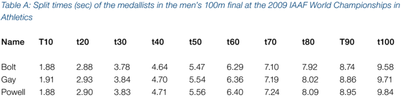
An example where the analysis of some aspects of the human body movement can be reduced to the analysis of a particle is the study of the Biomechanics of the 100-m race.
A technical report with the kinematic data for the 100-m world record by Usain Bolt can be downloaded from the website for Research Projects from the International Association of Athletics Federations.
Here is a direct link for that report. In particular, the following table shows the data for the three medalists in that race:
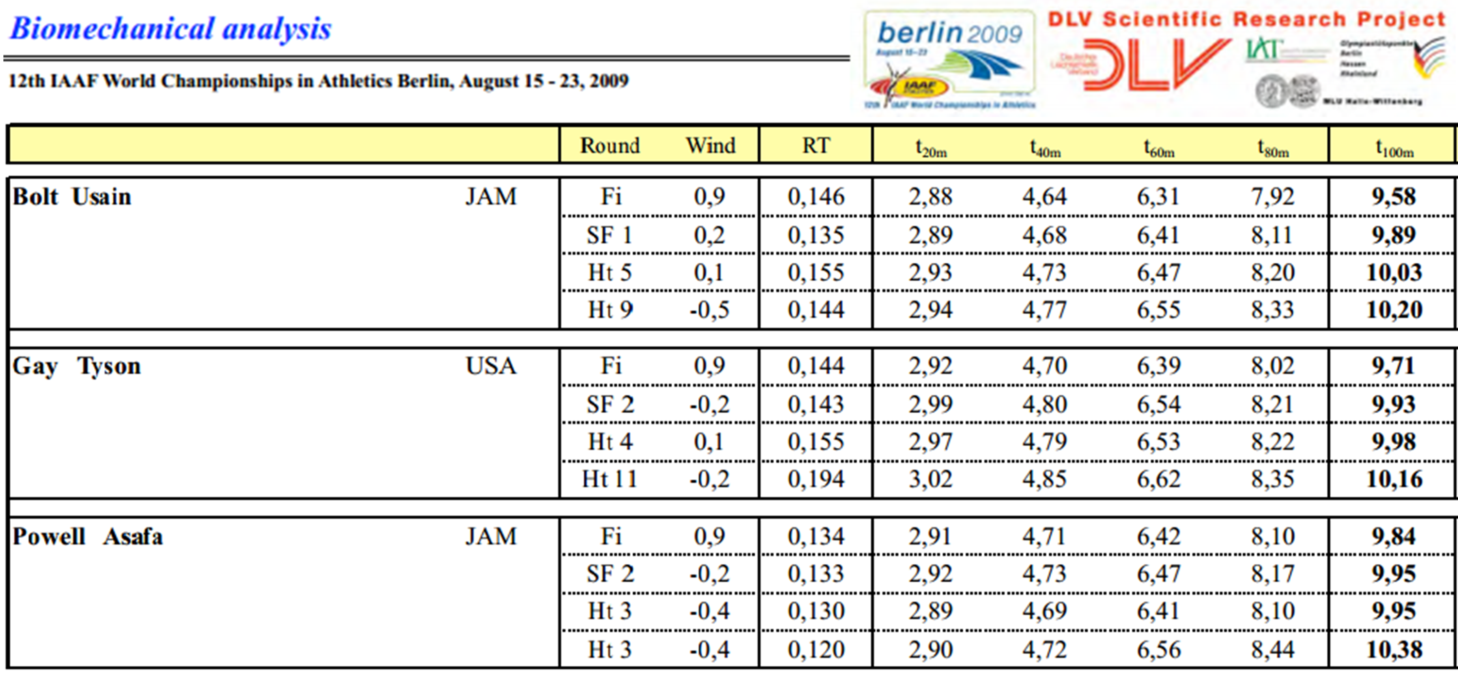
The column RT in the table above refers to the reaction time of each athlete. The IAAF has a very strict rule about reaction time: any athlete with a reaction time less than 100 ms is disqualified from the competition! See the website Reaction Times and Sprint False Starts for a discussion about this rule.
You can measure your own reaction time in a simple way visiting this website: http://www.humanbenchmark.com/tests/reactiontime.
The article A Kinematics Analysis Of Three Best 100 M Performances Ever by Krzysztof and Mero presents a detailed kinematic analysis of 100-m races.
Further reading
- Read the preface and first chapter of the Ruina and Rudra's book about how someone should study Mechanics.
- See the notebook Spatial and temporal characteristics about how the simple measurement of spatial and temporal kinematic variables can be very useful to describe the human gait.
- See the notebook The minimum jerk hypothesis about the conjecture that movements are performed (organized) with the smoothest trajectory possible.
Video lectures on the Internet
Problems
Answer the 12 questions of the Khan Academy's test on one-dimensional motion.
Consider the data for the three medalists of the 100-m dash in Berlin, 2009, shown previously.
a. Calculate the average velocity and acceleration.
b. Plot the graphs for the displacement, velocity, and acceleration versus time.
c. Plot the graphs velocity and acceleration versus partial distance (every 20m).
d. Calculate the average velocity and average acceleration and the instants and values of the peak velocity and peak acceleration.
- The article "Biomechanical Analysis of the Sprint and Hurdles Events at the 2009 IAAF World Championships in Athletics" by Graubner and Nixdorf lists the 10-m split times for the three medalists of the 100-m dash in Berlin, 2009:
a. Repeat the same calculations performed in problem 2 and compare the results.
- A body attached to a spring has its position (in cm) described by the equation $x(t) = 2\sin(4\pi t + \pi/4)$.
a. Calculate the equation for the body velocity and acceleration.
b. Plot the position, velocity, and acceleration in the interval [0, 1] s.
There are some nice free software that can be used for the kinematic analysis of human motion. Some of them are: Kinovea, Tracker, and SkillSpector. Visit their websites and explore these software to understand in which biomechanical applications they could be used.
From Ruina and Rudra's book, solve the problems 12.1.1 to 12.1.14.
References
- Graubner R, Nixdorf E (2011) Biomechanical Analysis of the Sprint and Hurdles Events at the 2009 IAAF World Championships in Athletics . New Studies in Athletics, 1/2, 19-53.
- Krzysztof M, Antti Mero A (2013) A Kinematics Analysis Of Three Best 100 M Performances Ever. Journal of Human Kinetics, 36, 149–160.
- Research Projects from the International Association of Athletics Federations.
- Ruina A, Rudra P (2019) Introduction to Statics and Dynamics. Oxford University Press.