Free-Body Diagram for particles
Renato Naville Watanabe
Laboratory of Biomechanics and Motor Control
Federal University of ABC, Brazil
Contents
- 1 Python setup
- 2 Free-Body Diagram
- 3 Steps to draw a free-body diagram (FBD)
- 4 Basic element and forces
- 5 Examples of free-body diagram
- 5.1 No force acting on the particle
- 5.2 Gravity force acting on the particle
- 5.3 Ground reaction force
- 5.4 Mass-spring system with horizontal movement
- 5.5 Linear spring in bidimensional movement at horizontal plane
- 5.6 Particle under action of gravity and linear air resistance
- 5.7 Particle under action of gravity and nonlinear air resistance
- 5.8 Linear spring and damping on bidimensional horizontal movement
- 5.9 Simple muscle model
- 5.3 Ground reaction force
- 6 Further reading
- 7 Video lectures on the internet
- 8 Problems
- 9 References
Python setup
import numpy as np
import matplotlib.pyplot as plt
import seaborn as sns
%matplotlib inline
sns.set_context('notebook', font_scale=1.2)
Free-Body Diagram
In the mechanical modeling of an inanimate or living system, composed by one or more bodies (bodies as units that are mechanically isolated according to the question one is trying to answer), it is convenient to isolate each body (be they originally interconnected or not) and identify each force and moment of force (torque) that act on this body in order to apply the laws of mechanics.
The free body diagram (FBD) of a mechanical system or model is the representation in a diagram of all forces and moments of force acting on each body, isolated from the rest of the system.
The term free means that each body, which maybe was part of a connected system, is represented as isolated (free) and any existent contact force is represented in the diagram as forces (action and reaction) acting on the formerly connected bodies. Then, the laws of mechanics are applied on each body, and the unknown movement, force or moment of force can be found if the system of equations is determined (the number of unknown variables can not be greater than the number of equations for each body).
How exactly a FBD is drawn for a mechanical model of something is dependent on what one is trying to find. For example, the air resistance might be neglected or not when modeling the movement of an object and the number of parts the system is divided is dependent on what is needed to know about the model.
The use of FBD is very common in biomechanics; a typical use is to use the FBD in order to determine the forces and torques on the ankle, knee, and hip joints of the lower limb (foot, leg, and thigh) during locomotion, and the FBD can be applied to any problem where the laws of mechanics are needed to solve a problem.
For now, let's study how to draw free-body diagrams for systems that can be modeled as particles.
Steps to draw a free-body diagram (FBD)
- Draw separately each object considered in the problem. How you separate depends on what questions you want to answer.
- Identify the forces acting on each object. If you are analyzing more than one object, remember the Newton's third Law (action and reaction), and identify where the reaction of a force is being applied.
- Draw all the identified forces, representing them as vectors. The vectors should be represented with the origin in the object. In the case of particles, the origin should be in the center of the particle.
- If necessary, you should represent the reference frame in the free-body diagram.
- After this, you can solve the problem using the Newton's second Law (see, e.g, Newton's Laws) to find the motion of the particle.
Basic element and forces
Gravity
The gravity force acts on two masses, each one atracting each other:
\begin{equation} \vec{{\bf{F}}} = - G\frac{m_1m_2}{||\vec{\bf{r}}||^2}\frac{\vec{\bf{r}}}{||\vec{\bf{r}}||} \end{equation}where $G = 6.67.10^{−11} Nm^2/kg^2$ and $\vec{\bf{r}}$ is a vector with length equal to the distance between the masses and directing towards the other mass. Note the forces acting on each mass have the same absolute value.
Since the mass of the Earth is $m_1=5.9736×10^{24}kg$ and its radius is 6.371×10$^6$ m, the gravity force near the surface of the Earth is:
\begin{equation} \vec{{\bf{F}}} = m\vec{\bf{g}} \end{equation}with the absolute value of $\vec{\bf{g}}$ approximately equal to 9.81 $m/s^2$, pointing towards the center of Earth.
Spring
Spring is an element used to represent a force proportional to some length or displacement. It produces a force in the same direction of the vector linking the spring extremities and opposite to its length or displacement from an equilibrium length. Frequently it has a linear relation, but it could be nonlinear as well. The force exerted by the spring in one of the extremities is:
\begin{equation} \vec{\bf{F}} = - k(||\vec{\bf{r}}||-l_0)\frac{\vec{\bf{r}}}{||\vec{\bf{r}}||} = -k\vec{\bf{r}} +kl_0\frac{\vec{\bf{r}}}{||\vec{\bf{r}}||} = -k\left(1-\frac{l_0}{||\vec{\bf{r}}||}\right)\vec{\bf{r}} \end{equation}where $\vec{\bf{r}}$ is the vector linking the extremity applying the force to the other extremity and $l_0$ is the equilibrium length of the spring.
Since the spring element is a massless element, the force in both extremities have the same absolute value and opposite directions.
Damping
Damper is an element used to represent a force proportional to the velocity of displacement. It produces a force in the opposite direction of its velocity.
Frequently it has a linear relation, but it could be nonlinear as well. The force exerted by the damper element in one of its extremities is:
\begin{equation} \vec{\bf{F}} = - b||\vec{\bf{v}}||\frac{\vec{\bf{v}}}{||\vec{\bf{v}}||} = -b\vec{\bf{v}} = -b\frac{d\vec{\bf{r}}}{dt} \end{equation}where $\vec{\bf{r}}$ is the vector linking the extremity applying the force to the other extremity.
Since the damper element is a massless element, , the force in both extremities have the same absolute value and opposite directions.
Examples of free-body diagram
Let's see some examples on how to draw the free-body diagram and obtain the motion equations to solve the problems.
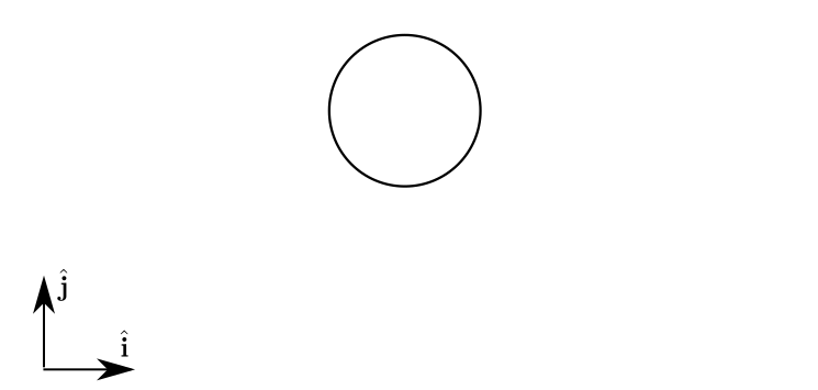
1. No force acting on the particle
The most trivial situation is a particle with no force acting on it.
The free-body diagram is below, with no force vectors acting on the particle.
In this situation, the resultant force is:
\begin{equation} \vec{\bf{F}} = 0 \end{equation}And the second Newton law for this particle is:
\begin{equation} m\frac{d^2\vec{\bf{r}}}{dt^2} = 0 \quad \rightarrow \quad \frac{d^2\vec{\bf{r}}}{dt^2} = 0 \end{equation}The motion of of the particle can be found by integrating twice both times, getting the following:
\begin{equation} \vec{\bf{r}} = \vec{\bf{v}}_0t + \vec{\bf{r}}_0 \end{equation}The particle continues to change its position with the same velocity it was at the beginning of the analysis. This could be predicted by Newton's first law.
2. Gravity force acting on the particle
Now, let's consider a ball with the gravity force acting on it. The free-body diagram is depicted below.
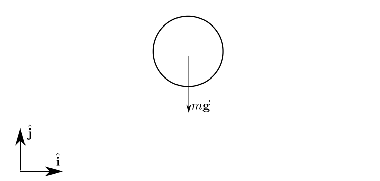
The only force acting on the ball is the gravitational force:
\begin{equation} \vec{\bf{F}}_g = - mg \; \hat{\bf{j}} \end{equation}Applying Newton's second Law:
\begin{equation} \vec{\bf{F}}_g = m \frac{d^2\vec{\bf{r}}}{dt^2} \rightarrow - mg \; \hat{\bf{j}} = m \frac{d^2\vec{\bf{r}}}{dt^2} \rightarrow - g \; \hat{\bf{j}} = \frac{d^2\vec{\bf{r}}}{dt^2} \end{equation}Now, we can separate the equation in two components (x and y):
\begin{equation} 0 = \frac{d^2x}{dt^2} \end{equation}and
\begin{equation} - g = \frac{d^2y}{dt^2} \end{equation}These equations were solved in this Notebook about the Newton's laws.
3. Ground reaction force
Now, we will analyze the situation of a particle at rest in contact with the ground. To simplify the analysis, only the vertical movement will be considered.
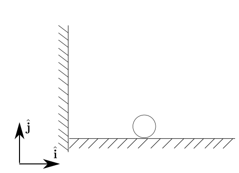
The forces acting on the particle are the ground reaction force (often called as normal force) and the gravity force. The free-body diagram of the particle is below:
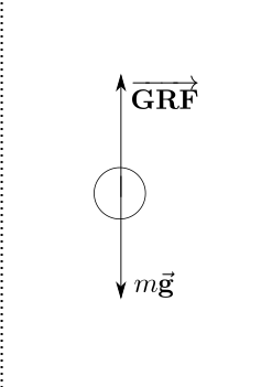
So, the resultant force in the particle is:
\begin{equation} \vec{\bf{F}} = \overrightarrow{\bf{GRF}} + m\vec{\bf{g}} = \overrightarrow{\bf{GRF}} - mg \; \hat{\bf{j}} \end{equation}Considering only the y direction:
\begin{equation} F = GRF - mg \end{equation}Applying Newton's second law to the particle:
\begin{equation} m \frac{d^2y}{dt^2} = GRF - mg \end{equation}Note that since we have no information about how the force GRF varies along time, we cannot solve this equation. To find the position of the particle along time, one would have to measure the ground reaction force. See the notebook on Vertical jump for an application of this model.
4. Mass-spring system with horizontal movement
The example below represents a mass attached to a spring and the other extremity of the spring is fixed.
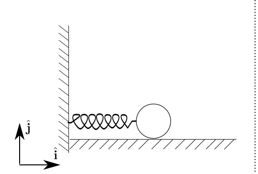
The only force force acting on the mass is from the spring. Below is the free-body diagram from the mass.
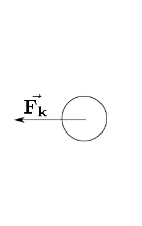
Since the movement is horizontal, we can neglect the gravity force.
\begin{equation} \vec{\bf{F}} = -k\left(1-\frac{l_0}{||\vec{\bf{r}}||}\right)\vec{\bf{r}} \end{equation}Applying Newton's second law to the mass:
\begin{equation} m\frac{d^2\vec{\bf{r}}}{dt^2} = -k\left(1-\frac{l_0}{||\vec{\bf{r}}||}\right)\vec{\bf{r}} \rightarrow \frac{d^2\vec{\bf{r}}}{dt^2} = -\frac{k}{m}\left(1-\frac{l_0}{||\vec{\bf{r}}||}\right)\vec{\bf{r}} \end{equation}Since the movement is unidimensional, we can deal with it scalarly:
\begin{equation} \frac{d^2x}{dt^2} = -\frac{k}{m}\left(1-\frac{l_0}{x}\right)x = -\frac{k}{m}(x-l_0) \end{equation}To solve this equation numerically, we must break the equations into two first-order differential equation:
\begin{equation} \frac{dv_x}{dt} = -\frac{k}{m}(x-l_0) \end{equation} \begin{equation} \frac{dx}{dt} = v_x \end{equation}In the numerical solution below, we will use $k = 40 N/m$, $m = 2 kg$, $l_0 = 0.5 m$ and the mass starts from the position $x = 0.8m$ and at rest.
k = 40
m = 2
l0 = 0.5
x0 = 0.8
v0 = 0

x = x0
v = v0

dt = 0.001
t = np.arange(0, 3, dt)

r = np.array([x])

for i in t[1:]:
    dxdt = v
    dvxdt = -k/m*(x-l0)
    x = x + dt*dxdt
    v = v + dt*dvxdt
    r = np.vstack((r,np.array([x])))

plt.figure(figsize=(8, 4))
plt.plot(t, r, lw=4)
plt.xlabel('t(s)')
plt.ylabel('x(m)')
plt.title('Spring displacement')
plt.show()

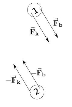
5. Linear spring in bidimensional movement at horizontal plane
This example below represents a system with two masses attached to a spring.
To solve the motion of both masses, we have to draw a free-body diagram for each one of the masses.
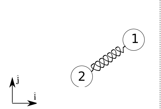
The only force acting on each mass is the force due to the spring. Since the movement is happening at the horizontal plane, the gravity force can be neglected.
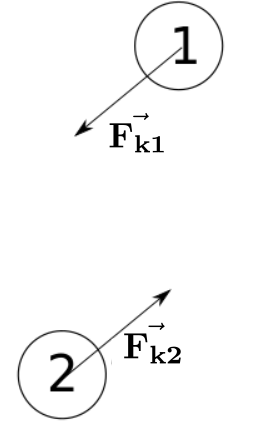
So, the forces acting on mass 1 is:
\begin{equation} \vec{\bf{F_1}} = k\left(||\vec{\bf{r_2}}-\vec{\bf{r_1}}||-l_0\right)\frac{(\vec{\bf{r_2}}-\vec{\bf{r_1}})}{||\vec{\bf{r_2}}-\vec{\bf{r_1}}||} \end{equation}and the forces acting on mass 2 is:
\begin{equation} \vec{\bf{F_2}} =k\left(||\vec{\bf{r_2}}-\vec{\bf{r_1}}||-l_0\right)\frac{(\vec{\bf{r_1}}-\vec{\bf{r_2}})}{||\vec{\bf{r_2}}-\vec{\bf{r_1}}||} \end{equation}Applying Newton's second law for the masses:
\begin{equation} m_1\frac{d^2\vec{\bf{r_1}}}{dt^2} = k\left(||\vec{\bf{r_2}}-\vec{\bf{r_1}}||-l_0\right)\frac{(\vec{\bf{r_2}}-\vec{\bf{r_1}})}{||\vec{\bf{r_2}}-\vec{\bf{r_1}}||} \\ \frac{d^2\vec{\bf{r_1}}}{dt^2} = -\frac{k}{m_1}\left(1-\frac{l_0}{||\vec{\bf{r_2}}-\vec{\bf{r_1}}||}\right)\vec{\bf{r_1}}+\frac{k}{m_1}\left(1-\frac{l_0}{||\vec{\bf{r_2}}-\vec{\bf{r_1}}||}\right)\vec{\bf{r_2}} \\ \frac{d^2x_1\hat{\bf{i}}}{dt^2}+\frac{d^2y_1\hat{\bf{j}}}{dt^2} = -\frac{k}{m_1}\left(1-\frac{l_0}{||\vec{\bf{r_2}}-\vec{\bf{r_1}}||}\right)(x_1\hat{\bf{i}}+y_1\hat{\bf{j}})+\frac{k}{m_1}\left(1-\frac{l_0}{||\vec{\bf{r_2}}-\vec{\bf{r_1}}||}\right)(x_2\hat{\bf{i}}+y_2\hat{\bf{j}}) \end{equation}\begin{equation} m_2\frac{d^2\vec{\bf{r_2}}}{dt^2} = k\left(||\vec{\bf{r_2}}-\vec{\bf{r_1}}||-l_0\right)\frac{(\vec{\bf{r_1}}-\vec{\bf{r_2}})}{||\vec{\bf{r_2}}-\vec{\bf{r_1}}||} \\ \frac{d^2\vec{\bf{r_2}}}{dt^2} = -\frac{k}{m_2}\left(1-\frac{l_0}{||\vec{\bf{r_2}}-\vec{\bf{r_1}}||}\right)\vec{\bf{r_2}}+\frac{k}{m_2}\left(1-\frac{l_0}{||\vec{\bf{r_2}}-\vec{\bf{r_1}}||}\right)\vec{\bf{r_1}} \\ \frac{d^2x_2\hat{\bf{i}}}{dt^2}+\frac{d^2y_2\hat{\bf{j}}}{dt^2} = -\frac{k}{m_2}\left(1-\frac{l_0}{||\vec{\bf{r_2}}-\vec{\bf{r_1}}||}\right)(x_2\hat{\bf{i}}+y_2\hat{\bf{j}})+\frac{k}{m_2}\left(1-\frac{l_0}{||\vec{\bf{r_2}}-\vec{\bf{r_1}}||}\right)(x_1\hat{\bf{i}}+y_1\hat{\bf{j}}) \end{equation}
Now, we can separate the equations for each of the coordinates:
\begin{equation} \frac{d^2x_1}{dt^2} = -\frac{k}{m_1}\left(1-\frac{l_0}{||\vec{\bf{r_2}}-\vec{\bf{r_1}}||}\right)x_1+\frac{k}{m_1}\left(1-\frac{l_0}{||\vec{\bf{r_2}}-\vec{\bf{r_1}}||}\right)x_2=-\frac{k}{m_1}\left(1-\frac{l_0}{\sqrt{(x_2-x_1)^2+(y_2-y_1)^2}}\right)(x_1-x_2) \end{equation} \begin{equation} \frac{d^2y_1}{dt^2} = -\frac{k}{m_1}\left(1-\frac{l_0}{||\vec{\bf{r_2}}-\vec{\bf{r_1}}||}\right)y_1+\frac{k}{m_1}\left(1-\frac{l_0}{||\vec{\bf{r_2}}-\vec{\bf{r_1}}||}\right)y_2=-\frac{k}{m_1}\left(1-\frac{l_0}{\sqrt{(x_2-x_1)^2+(y_2-y_1)^2}}\right)(y_1-y_2) \end{equation} \begin{equation} \frac{d^2x_2}{dt^2} = -\frac{k}{m_2}\left(1-\frac{l_0}{||\vec{\bf{r_2}}-\vec{\bf{r_1}}||}\right)x_2+\frac{k}{m_2}\left(1-\frac{l_0}{||\vec{\bf{r_2}}-\vec{\bf{r_1}}||}\right)x_1=-\frac{k}{m_2}\left(1-\frac{l_0}{\sqrt{(x_2-x_1)^2+(y_2-y_1)^2}}\right)(x_2-x_1) \end{equation} \begin{equation} \frac{d^2y_2}{dt^2} = -\frac{k}{m_2}\left(1-\frac{l_0}{||\vec{\bf{r_2}}-\vec{\bf{r_1}}||}\right)y_2+\frac{k}{m_2}\left(1-\frac{l_0}{||\vec{\bf{r_2}}-\vec{\bf{r_1}}||}\right)y_1=-\frac{k}{m_2}\left(1-\frac{l_0}{\sqrt{(x_2-x_1)^2+(y_2-y_1)^2}}\right)(y_2-y_1) \end{equation}To solve these equations numerically, you must break these equations into first-order equations:
\begin{equation} \frac{dv_{x_1}}{dt} = -\frac{k}{m_1}\left(1-\frac{l_0}{\sqrt{(x_2-x_1)^2+(y_2-y_1)^2}}\right)(x_1-x_2) \end{equation} \begin{equation} \frac{dv_{y_1}}{dt} = -\frac{k}{m_1}\left(1-\frac{l_0}{\sqrt{(x_2-x_1)^2+(y_2-y_1)^2}}\right)(y_1-y_2) \end{equation} \begin{equation} \frac{dv_{x_2}}{dt} = -\frac{k}{m_2}\left(1-\frac{l_0}{\sqrt{(x_2-x_1)^2+(y_2-y_1)^2}}\right)(x_2-x_1) \end{equation} \begin{equation} \frac{dv_{y_2}}{dt} = -\frac{k}{m_2}\left(1-\frac{l_0}{\sqrt{(x_2-x_1)^2+(y_2-y_1)^2}}\right)(y_2-y_1) \end{equation} \begin{equation} \frac{dx_1}{dt} = v_{x_1} \end{equation} \begin{equation} \frac{dy_1}{dt} = v_{y_1} \end{equation} \begin{equation} \frac{dx_2}{dt} = v_{x_2} \end{equation} \begin{equation} \frac{dy_2}{dt} = v_{y_2} \end{equation}Note that if you did not want to know the details about the motion of each mass, but only the motion of the center of mass of the masses-spring system, you could have modeled the whole system as a single particle.
To solve the equations numerically, we will use the $m_1=1 kg$, $m_2 = 2 kg$, $l_0 = 0.5 m$, $k = 90 N/m$ and $x_{1_0} = 0 m$, $x_{2_0} = 0 m$, $y_{1_0} = 1 m$, $y_{2_0} = -1 m$, $v_{x1_0} = -2 m/s$, $v_{x2_0} = 0 m/s$, $v_{y1_0} = 0 m/s$, $v_{y2_0} = 0 m/s$.
x01 = 0
y01= 0.5
x02 = 0
y02 = -0.5
vx01 = 0.1
vy01 = 0
vx02 = -0.1
vy02 = 0

x1= x01
y1 = y01
x2= x02
y2 = y02
vx1= vx01
vy1 = vy01
vx2= vx02
vy2 = vy02
r1 = np.array([x1,y1])
r2 = np.array([x2,y2])

k = 30
m1 = 1
m2 = 1
l0 = 0.5

dt = 0.0001
t = np.arange(0,5,dt)

for i in t[1:]:

    dvx1dt = -k/m1*(x1-x2)*(1-l0/np.sqrt((x2-x1)**2+(y2-y1)**2))
    dvx2dt = -k/m2*(x2-x1)*(1-l0/np.sqrt((x2-x1)**2+(y2-y1)**2))
    dvy1dt = -k/m1*(y1-y2)*(1-l0/np.sqrt((x2-x1)**2+(y2-y1)**2))
    dvy2dt = -k/m2*(y2-y1)*(1-l0/np.sqrt((x2-x1)**2+(y2-y1)**2))

    dx1dt = vx1
    dx2dt = vx2
    dy1dt = vy1
    dy2dt = vy2

    x1 = x1 + dt*dx1dt
    x2 = x2 + dt*dx2dt
    y1 = y1 + dt*dy1dt
    y2 = y2 + dt*dy2dt

    vx1 = vx1 + dt*dvx1dt
    vx2 = vx2 + dt*dvx2dt
    vy1 = vy1 + dt*dvy1dt
    vy2 = vy2 + dt*dvy2dt

    r1 = np.vstack((r1,np.array([x1,y1])))
    r2 = np.vstack((r2,np.array([x2,y2])))

springLength = np.sqrt((r1[:,0]-r2[:,0])**2+(r1[:,1]-r2[:,1])**2)
plt.figure(figsize=(8, 4))
plt.plot(t, springLength, lw=4)
plt.xlabel('t(s)')
plt.ylabel('Spring length (m)')
plt.show()

plt.figure(figsize=(8, 4))
plt.plot(r1[:,0], r1[:,1], 'r.', lw=4)
plt.plot(r2[:,0], r2[:,1], 'b.', lw=4)
plt.plot((m1*r1[:,0]+m2*r2[:,0])/(m1+m2), (m1*r1[:,1]+m2*r2[:,1])/(m1+m2),'g.')
plt.xlim(-0.7,0.7)
plt.ylim(-0.7,0.7)
plt.xlabel('x(m)')
plt.ylabel('y(m)')
plt.title('Masses position')
plt.legend(('Mass1','Mass 2','Masses center of mass'))
plt.show()


6. Particle under action of gravity and linear air resistance
Below is the free-body diagram of a particle with the gravity force and a linear drag force due to the air resistance.
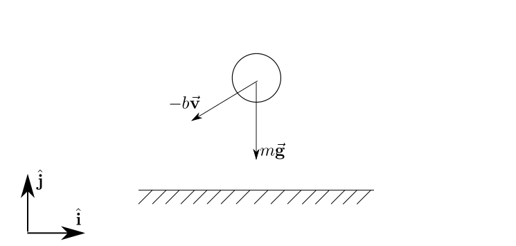
the forces being applied in the ball are:
\begin{equation} \vec{\bf{F}} = -mg \hat{\bf{j}} - b\vec{\bf{v}} = -mg \hat{\bf{j}} - b\frac{d\vec{\bf{r}}}{dt} = -mg \hat{\bf{j}} - b\left(\frac{dx}{dt}\hat{\bf{i}}+\frac{dy}{dt}\hat{\bf{j}}\right) = - b\frac{dx}{dt}\hat{\bf{i}} - \left(mg + b\frac{dy}{dt}\right)\hat{\bf{j}} \end{equation}Writing down Newton's second law:
\begin{equation} \vec{\bf{F}} = m \frac{d^2\vec{\bf{r}}}{dt^2} \rightarrow - b\frac{dx}{dt}\hat{\bf{i}} - \left(mg + b\frac{dy}{dt}\right)\hat{\bf{j}} = m\left(\frac{d^2x}{dt^2}\hat{\bf{i}}+\frac{d^2y}{dt^2}\hat{\bf{j}}\right) \end{equation}Now, we can separate into one equation for each coordinate:
\begin{equation} - b\frac{dx}{dt} = m\frac{d^2x}{dt^2} -\rightarrow \frac{d^2x}{dt^2} = -\frac{b}{m} \frac{dx}{dt} \end{equation} \begin{equation} -mg - b\frac{dy}{dt} = m\frac{d^2y}{dt^2} \rightarrow \frac{d^2y}{dt^2} = -\frac{b}{m}\frac{dy}{dt} - g \end{equation}These equations were solved in this notebook.
7. Particle under action of gravity and nonlinear air resistance
Below, is the free-body diagram of a particle with the gravity force and a drag force due to the air resistance proportional to the square of the particle velocity.
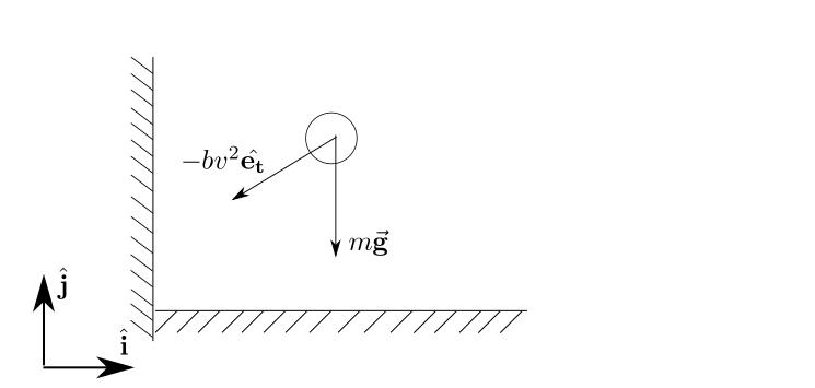
The forces being applied in the ball are:
\begin{equation} \vec{\bf{F}} = -mg \hat{\bf{j}} - bv^2\hat{\bf{e_t}} = -mg \hat{\bf{j}} - b (v_x^2+v_y^2) \frac{v_x\hat{\bf{i}}+v_y\hat{\bf{j}}}{\sqrt{v_x^2+v_y^2}} = -mg \hat{\bf{j}} - b \sqrt{v_x^2+v_y^2} \,(v_x\hat{\bf{i}}+v_y\hat{\bf{j}}) = -mg \hat{\bf{j}} - b \sqrt{\left(\frac{dx}{dt} \right)^2+\left(\frac{dy}{dt} \right)^2} \,\left(\frac{dx}{dt} \hat{\bf{i}}+\frac{dy}{dt}\hat{\bf{j}}\right) \end{equation}Writing down Newton's second law:
\begin{equation} \vec{\bf{F}} = m \frac{d^2\vec{\bf{r}}}{dt^2} \rightarrow -mg \hat{\bf{j}} - b \sqrt{\left(\frac{dx}{dt} \right)^2+\left(\frac{dy}{dt} \right)^2} \,\left(\frac{dx}{dt} \hat{\bf{i}}+\frac{dy}{dt}\hat{\bf{j}}\right) = m\left(\frac{d^2x}{dt^2}\hat{\bf{i}}+\frac{d^2y}{dt^2}\hat{\bf{j}}\right) \end{equation}Now, we can separate into one equation for each coordinate:
\begin{equation} - b \sqrt{\left(\frac{dx}{dt} \right)^2+\left(\frac{dy}{dt} \right)^2} \,\frac{dx}{dt} = m\frac{d^2x}{dt^2} \rightarrow \frac{d^2x}{dt^2} = - \frac{b}{m} \sqrt{\left(\frac{dx}{dt} \right)^2+\left(\frac{dy}{dt} \right)^2} \,\frac{dx}{dt} \end{equation} \begin{equation} -mg - b \sqrt{\left(\frac{dx}{dt} \right)^2+\left(\frac{dy}{dt} \right)^2} \,\frac{dy}{dt} = m\frac{d^2y}{dt^2} \rightarrow \frac{d^2y}{dt^2} = - \frac{b}{m} \sqrt{\left(\frac{dx}{dt} \right)^2+\left(\frac{dy}{dt} \right)^2} \,\frac{dy}{dt} -g \end{equation}These equations were solved numerically in this notebook.
8. Linear spring and damping on bidimensional horizontal movement
This situation is very similar to the example of horizontal movement with one spring and two masses, with a damper added in parallel to the spring.
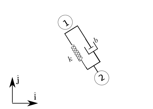
Now, the forces acting on each mass are the force due to the spring and the force due to the damper.
So, the forces acting on mass 1 is:
\begin{equation} \vec{\bf{F_1}} = b\frac{d(\vec{\bf{r_2}}-\vec{\bf{r_1}})}{dt} + k\left(||\vec{\bf{r_2}}-\vec{\bf{r_1}}||-l_0\right)\frac{(\vec{\bf{r_2}}-\vec{\bf{r_1}})}{||\vec{\bf{r_2}}-\vec{\bf{r_1}}||} = b\frac{d(\vec{\bf{r_2}}-\vec{\bf{r_1}})}{dt} + k\left(1-\frac{l_0}{||\vec{\bf{r_2}}-\vec{\bf{r_1}}||}\right)(\vec{\bf{r_2}}-\vec{\bf{r_1}}) \end{equation}and the forces acting on mass 2 is:
\begin{equation} \vec{\bf{F_2}} = b\frac{d(\vec{\bf{r_1}}-\vec{\bf{r_2}})}{dt} + k\left(||\vec{\bf{r_2}}-\vec{\bf{r_1}}||-l_0\right)\frac{(\vec{\bf{r_1}}-\vec{\bf{r_2}})}{||\vec{\bf{r_1}}-\vec{\bf{r_2}}||}= b\frac{d(\vec{\bf{r_1}}-\vec{\bf{r_2}})}{dt} + k\left(1-\frac{l_0}{||\vec{\bf{r_2}}-\vec{\bf{r_1}}||}\right)(\vec{\bf{r_1}}-\vec{\bf{r_2}}) \end{equation}Applying the Newton's second law for the masses:
\begin{equation} m_1\frac{d^2\vec{\bf{r_1}}}{dt^2} = b\frac{d(\vec{\bf{r_2}}-\vec{\bf{r_1}})}{dt}+k\left(1-\frac{l_0}{||\vec{\bf{r_2}}-\vec{\bf{r_1}}||}\right)(\vec{\bf{r_2}}-\vec{\bf{r_1}}) \end{equation} \begin{equation} \frac{d^2\vec{\bf{r_1}}}{dt^2} = -\frac{b}{m_1}\frac{d\vec{\bf{r_1}}}{dt} -\frac{k}{m_1}\left(1-\frac{l_0}{||\vec{\bf{r_2}}-\vec{\bf{r_1}}||}\right)\vec{\bf{r_1}} + \frac{b}{m_1}\frac{d\vec{\bf{r_2}}}{dt}+\frac{k}{m_1}\left(1-\frac{l_0}{||\vec{\bf{r_2}}-\vec{\bf{r_1}}||}\right)\vec{\bf{r_2}} \end{equation} \begin{equation} \frac{d^2x_1\hat{\bf{i}}}{dt^2}+\frac{d^2y_1\hat{\bf{j}}}{dt^2} = -\frac{b}{m_1}\left(\frac{dx_1\hat{\bf{i}}}{dt}+\frac{dy_1\hat{\bf{j}}}{dt}\right)-\frac{k}{m_1}\left(1-\frac{l_0}{||\vec{\bf{r_2}}-\vec{\bf{r_1}}||}\right)(x_1\hat{\bf{i}}+y_1\hat{\bf{j}})+\frac{b}{m_1}\left(\frac{dx_2\hat{\bf{i}}}{dt}+\frac{dy_2\hat{\bf{j}}}{dt}\right)+\frac{k}{m_1}\left(1-\frac{l_0}{||\vec{\bf{r_2}}-\vec{\bf{r_1}}||}\right)(x_2\hat{\bf{i}}+y_2\hat{\bf{j}}) = -\frac{b}{m_1}\left(\frac{dx_1\hat{\bf{i}}}{dt}+\frac{dy_1\hat{\bf{j}}}{dt}-\frac{dx_2\hat{\bf{i}}}{dt}-\frac{dy_2\hat{\bf{j}}}{dt}\right)-\frac{k}{m_1}\left(1-\frac{l_0}{\sqrt{(x_2-x_1)^2+(y_2-y_1)^2}}\right)(x_1\hat{\bf{i}}+y_1\hat{\bf{j}}-x_2\hat{\bf{i}}-y_2\hat{\bf{j}}) \end{equation}Now, we can separate the equations for each of the coordinates:
\begin{equation} \frac{d^2x_1}{dt^2} = -\frac{b}{m_1}\left(\frac{dx_1}{dt}-\frac{dx_2}{dt}\right)-\frac{k}{m_1}\left(1-\frac{l_0}{\sqrt{(x_2-x_1)^2+(y_2-y_1)^2}}\right)(x_1-x_2) \end{equation} \begin{equation} \frac{d^2y_1}{dt^2} = -\frac{b}{m_1}\left(\frac{dy_1}{dt}-\frac{dy_2}{dt}\right)-\frac{k}{m_1}\left(1-\frac{l_0}{\sqrt{(x_2-x_1)^2+(y_2-y_1)^2}}\right)(y_1-y_2) \end{equation} \begin{equation} \frac{d^2x_2}{dt^2} = -\frac{b}{m_2}\left(\frac{dx_2}{dt}-\frac{dx_1}{dt}\right)-\frac{k}{m_2}\left(1-\frac{l_0}{\sqrt{(x_2-x_1)^2+(y_2-y_1)^2}}\right)(x_2-x_1) \end{equation} \begin{equation} \frac{d^2y_2}{dt^2} = -\frac{b}{m_2}\left(\frac{dy_2}{dt}-\frac{dy_1}{dt}\right)-\frac{k}{m_2}\left(1-\frac{l_0}{\sqrt{(x_2-x_1)^2+(y_2-y_1)^2}}\right)(y_2-y_1) \end{equation}If you want to solve these equations numerically, you must break these equations into first-order equations:
\begin{equation} \frac{dv_{x_1}}{dt} = -\frac{b}{m_1}\left(v_{x_1}-v_{x_2}\right)-\frac{k}{m_1}\left(1-\frac{l_0}{\sqrt{(x_2-x_1)^2+(y_2-y_1)^2}}\right)(x_1-x_2) \end{equation} \begin{equation} \frac{dv_{y_1}}{dt} = -\frac{b}{m_1}\left(v_{y_1}-v_{y_2}\right)-\frac{k}{m_1}\left(1-\frac{l_0}{\sqrt{(x_2-x_1)^2+(y_2-y_1)^2}}\right)(y_1-y_2) \end{equation} \begin{equation} \frac{dv_{x_2}}{dt} = -\frac{b}{m_2}\left(v_{x_2}-v_{x_1}\right)-\frac{k}{m_2}\left(1-\frac{l_0}{\sqrt{(x_2-x_1)^2+(y_2-y_1)^2}}\right)(x_2-x_1) \end{equation} \begin{equation} \frac{dv_{y_2}}{dt} = -\frac{b}{m_2}\left(v_{y_2}-v_{y_1}\right)-\frac{k}{m_2}\left(1-\frac{l_0}{\sqrt{(x_2-x_1)^2+(y_2-y_1)^2}}\right)(y_2-y_1) \end{equation} \begin{equation} \frac{dx_1}{dt} = v_{x_1} \end{equation} \begin{equation} \frac{dy_1}{dt} = v_{y_1} \end{equation} \begin{equation} \frac{dx_2}{dt} = v_{x_2} \end{equation} \begin{equation} \frac{dy_2}{dt} = v_{y_2} \end{equation}To solve the equations numerically, we will use the $m_1=1 kg$, $m_2 = 2 kg$, $l_0 = 0.5 m$, $k = 10 N/m$, $b = 0.6 Ns/m$ and $x_{1_0} = 0 m$, $x_{2_0} = 0 m$, $y_{1_0} = 1 m$, $y_{2_0} = -1 m$, $v_{x1_0} = -2 m/s$, $v_{x2_0} = 1 m/s$, $v_{y1_0} = 0 m/s$, $v_{y2_0} = 0 m/s$.
x01 = 0
y01= 1
x02 = 0
y02 = -1

vx01 = -2
vy01 = 0
vx02 = 1
vy02 = 0

x1= x01
y1 = y01
x2= x02
y2 = y02
vx1= vx01
vy1 = vy01
vx2= vx02
vy2 = vy02
r1 = np.array([x1,y1])
r2 = np.array([x2,y2])

k = 10
m1 = 1
m2 = 2
b = 0.6
l0 = 0.5

dt = 0.001
t = np.arange(0,5,dt)

for i in t[1:]:
    dvx1dt = -b/m1*(vx1-vx2) -k/m1*(1-l0/np.sqrt((x2-x1)**2+(y2-y1)**2))*(x1-x2)
    dvx2dt = -b/m2*(vx2-vx1) -k/m2*(1-l0/np.sqrt((x2-x1)**2+(y2-y1)**2))*(x2-x1)
    dvy1dt = -b/m1*(vy1-vy2) -k/m1*(1-l0/np.sqrt((x2-x1)**2+(y2-y1)**2))*(y1-y2)
    dvy2dt = -b/m2*(vy2-vy1) -k/m2*(1-l0/np.sqrt((x2-x1)**2+(y2-y1)**2))*(y2-y1)
    dx1dt = vx1
    dx2dt = vx2
    dy1dt = vy1
    dy2dt = vy2
    x1 = x1 + dt*dx1dt
    x2 = x2 + dt*dx2dt
    y1 = y1 + dt*dy1dt
    y2 = y2 + dt*dy2dt
    vx1 = vx1 + dt*dvx1dt
    vx2 = vx2 + dt*dvx2dt
    vy1 = vy1 + dt*dvy1dt
    vy2 = vy2 + dt*dvy2dt
    r1 = np.vstack((r1,np.array([x1,y1])))
    r2 = np.vstack((r2,np.array([x2,y2])))

springDampLength = np.sqrt((r1[:,0]-r2[:,0])**2+(r1[:,1]-r2[:,1])**2)

plt.figure(figsize=(8, 4))
plt.plot(t, springDampLength, lw=4)
plt.xlabel('t(s)')
plt.ylabel('Spring length (m)')
plt.show()

plt.figure(figsize=(8, 4))
plt.plot(r1[:,0], r1[:,1], 'r.', lw=4)
plt.plot(r2[:,0], r2[:,1], 'b.', lw=4)
plt.plot((m1*r1[:,0]+m2*r2[:,0])/(m1+m2), (m1*r1[:,1]+m2*r2[:,1])/(m1+m2),'g.')
plt.xlim(-2,2)
plt.ylim(-2,2)
plt.xlabel('x(m)')
plt.ylabel('y(m)')
plt.title('Masses position')
plt.legend(('Mass1','Mass 2','Masses center of mass'))
plt.show()


9. Simple muscle model
The diagram below shows a simple muscle model. The spring in the left represents the tendinous tissues and the spring in the right represents the elastic properties of the muscle fibers. The damping is present to model the viscous properties of the muscle fibers, the element CE is the contractile element (force production) and the mass $m$ is the muscle mass.
The length $L_{MT}$ is the length of the muscle plus the tendon. In our model $L_{MT}$ is constant, but it could be a function of the joint angle.
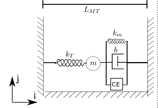
The length of the tendon will be denoted by $l_T(t)$ and the muscle length, by $l_{m}(t)$. Both lengths are related by each other by the following expression:
\begin{equation} l_t(t) + l_m(t) = L_{MT} \end{equation}The free-body diagram of the muscle mass is depicted below.
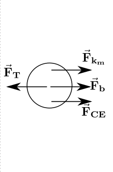
The resultant force being applied in the muscle mass is:
$$\vec{\bf{F}} = -k_T(||\vec{\bf{r_m}}||-l_{t_0})\frac{\vec{\bf{r_m}}}{||\vec{\bf{r_m}}||} + b\frac{d(L_{MT}\hat{\bf{i}} - \vec{\bf{r_{m}}})}{dt} + k_m (||L_{MT}\hat{\bf{i}} - \vec{\bf{r_{m}}}||-l_{m_0})\frac{L_{MT}\hat{\bf{i}} - \vec{\bf{r_{m}}}}{||L_{MT}\hat{\bf{i}} - \vec{\bf{r_{m}}}||} +\vec{\bf{F}}{\bf{_{CE}}}(t)$$where $\vec{\bf{r_m}}$ is the muscle mass position.
Since the model is unidimensional, we can assume that the force $\vec{\bf{F}}\bf{_{CE}}(t)$ is in the x direction, so the analysis will be done only in this direction.
$$F = -k_T(l_t-l_{t_0}) + b\frac{d(L_{MT} - l_t)}{dt} + k_m (l_m-l_{m_0}) + F_{CE}(t) \\ F = -k_T(l_t-l_{t_0}) -b\frac{dl_t}{dt} + k_m (L_{MT}-l_t-l_{m_0}) + F_{CE}(t) \\ F = -b\frac{dl_t}{dt}-(k_T+k_m)l_t+F_{CE}(t)+k_Tl_{t_0}+k_m(L_{MT}-l_{m_0})$$Applying the Newton's second law:
$$m\frac{d^2l_t}{dt^2} = -b\frac{dl_t}{dt}-(k_T+k_m)l_t+F_{CE}(t)+k_Tl_{t_0}+k_m(L_{MT}-l_{m_0})$$To solve this equation, we must break the equation into two first-order differential equations:
\begin{equation} \frac{dvt}{dt} = - \frac{b}{m}v_t - \frac{k_T+k_m}{m}l_t +\frac{F_{CE}(t)}{m} + \frac{k_T}{m}l_{t_0}+\frac{k_m}{m}(L_{MT}-l_{m_0}) \end{equation} \begin{equation} \frac{d l_t}{dt} = v_t \end{equation}Now, we can solve these equations by using some numerical method. To obtain the solution, we will use the damping factor of the muscle as $b = 10\,Ns/m$, the muscle mass is $m = 2 kg$, the stiffness of the tendon as $k_t=1000\,N/m$ and the elastic element of the muscle as $k_m=1500\,N/m$. The tendon-length is $L_{MT} = 0.35\,m$, and the tendon equilibrium length is $l_{t0} = 0.28\,m$ and the muscle fiber equilibrium length is $l_{m0} = 0.07\,m$. Both the tendon and the muscle fiber are at their equilibrium lengths and at rest.
Also, we will model the force of the contractile element as a Heaviside step of $90\,N$ (90 N beginning at $t=0$), but normally it is modeled as a function of $l_m$ and $v_m$ having a neural activation signal as input.
m = 2
b = 10
km = 1500
kt = 1000
lt0 = 0.28
lm0 = 0.07

Lmt = 0.35
vt0 = 0

dt = 0.0001
t = np.arange(0, 10, dt)

Fce = 90

lt = lt0
vt = vt0
ltp = np.array([lt0])
lmp = np.array([lm0])
Ft = np.array([0])
for i in range(1,len(t)):
    dvtdt = -b/m*vt-(kt+km)/m*lt  + Fce/m + kt/m*lt0 +km/m*(Lmt-lm0)
    dltdt = vt
    vt = vt + dt*dvtdt
    lt = lt + dt*dltdt
    Ft = np.vstack((Ft,np.array(kt*(lt-lt0))))
    ltp = np.vstack((ltp,np.array(lt)))
    lmp = np.vstack((lmp,np.array(Lmt - lt)))

plt.figure(figsize=(8, 4))
plt.plot(t, Ft, lw=4)
plt.xlabel('t(s)')
plt.ylabel('Tendon force (N)')
plt.show()
plt.figure(figsize=(8, 4))
plt.plot(t, ltp, lw=4)
plt.plot(t, lmp, lw=4)
plt.xlabel('t(s)')
plt.ylabel('Length (m)')
plt.legend(('Tendon length', 'Muscle fiber length'))
plt.show()


Further reading
- Read the 2nd chapter of the Ruina and Rudra's book about free-body diagrams;
- Read the 13th of the Hibbeler's book (available in the Classroom).
Problems
Draw free-body diagram for (see answers at https://youtu.be/3rZR7FSSidc):
- A book is at rest on a table.
- A book is attached to a string and hanging from the ceiling.
- A person pushes a crate to the right across a floor at a constant speed.
- A skydiver is falling downward a speeding up.
- A rightward-moving car has locked wheels and is skidding to a stop.
- A freight elevator is attached by a cable, being pulled upward, and slowing down. It is not touching the sides of the elevator shaft.
A block (2) is stacked on top of block (1) which is at rest on a surface (all contacts have friction). Which is the maximum horizontal force that can be applied to the block (1) such that block (2) does not slip? Answer at https://youtu.be/63U4_OxohOw
Consider two masses m1 = 5 kg and m2 = 3 kg attached to a pulley which is attached to a wall with a rope and m1 is pulled in the opposite direction with force F = 100 N as shown in the figure below. Calculate (Answer at https://youtu.be/Dgg76vNChEU):
- Friction force on m1
- Friction force on m2
- Tension on the rope attached to masses m1 and m2
- Acceleration of m1

- (Example 13.4 of Hibbeler's book) A smooth 2-kg collar C, shown in the figure below, is attached to a spring having a stiffness k = 3 N/m and an unstretched length of 0.75 m. If the collar is released from rest at A, determine its acceleration and the normal force of the rod on the collar at the instant y = 1 m.

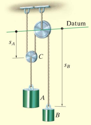
- (Example 13.5 of Hibbeler's book) The 100-kg block A shown in the figure below is released from rest. If the masses of the pulleys and the cord are neglected, determine the speed of the 20-kg block B in 2 s.
- (Example 13.9 of Hibbeler's book) The 60-kg skateboarder in the figure below coasts down the circular track. If he starts from rest when e = 0$^o$, determine the magnitude of the normal reaction the track exerts on him when e = 60$^o$. Neglect his size for the calculation.

- Solve the problems 2.3.9, 2.3.20, 11.1.6, 13.1.6 (a, b, c, d, f), 13.1.7, 13.1.10 (a, b) from Ruina and Pratap's book.
References
- Ruina A, Rudra P (2019) Introduction to Statics and Dynamics. Oxford University Press.
- R. C. Hibbeler (2010) Engineering Mechanics Dynamics. 12th Edition. Pearson Prentice Hall.
- Nigg & Herzog (2006) Biomechanics of the Musculo-skeletal System. 3rd Edition. Wiley.