Data enrichment
Introduction
We define enrichment as the process of augmenting your data with new variables by means of a spatial join between your data and a Dataset aggregated at a given spatial resolution in the CARTO Data Observatory, or in other words:
"Enrichment is the process of adding variables to a geometry, which we call the target, (point, line, polygon…) from a spatial (polygon) dataset, which we call the source"
We recommend you check out the CARTOframes quickstart since this guide uses some of the generated DataFrames as well as the Data Discovery guide to learn about exploring the Data Observatory catalog to find variables of interest for your analyses.
Choose variables to enrich from the Data Observatory catalog
Let's follow up with the Data Discovery guide, where we subscribed to the AGS demographics dataset and listed the variables available to enrich our own data.
from cartoframes.auth import set_default_credentials

set_default_credentials('creds.json')
from cartoframes.data.observatory import Catalog, Dataset, Variable, Geography
Catalog().subscriptions().datasets
[<Dataset.get('ags_businesscou_df363a87')>,
 <Dataset.get('ags_retailpoten_aaf25a8c')>,
 <Dataset.get('ags_sociodemogr_e92b1637')>,
 <Dataset.get('ags_crimerisk_e9cfa4d4')>]
dataset = Dataset.get('ags_sociodemogr_e92b1637')
variables = dataset.variables
variables
[<Variable.get('HINCYMED65_310bc888')> #'Median Household Income: Age 65-74 (2019A)',
 <Variable.get('HINCYMED55_1a269b4b')> #'Median Household Income: Age 55-64 (2019A)',
 <Variable.get('HINCYMED45_33daa0a')> #'Median Household Income: Age 45-54 (2019A)',
 <Variable.get('HINCYMED35_4c7c3ccd')> #'Median Household Income: Age 35-44 (2019A)',
 <Variable.get('HINCYMED25_55670d8c')> #'Median Household Income: Age 25-34 (2019A)',
 <Variable.get('HINCYMED24_22603d1a')> #'Median Household Income: Age < 25 (2019A)',
 <Variable.get('HINCYGT200_e552a738')> #'Household Income > $200000 (2019A)',
 <Variable.get('HINCY6075_1933e114')> #'Household Income $60000-$74999 (2019A)',
 <Variable.get('HINCY4550_f7ad7d79')> #'Household Income $45000-$49999 (2019A)',
 <Variable.get('HINCY4045_98177a5c')> #'Household Income $40000-$44999 (2019A)',
 <Variable.get('HINCY3540_73617481')> #'Household Income $35000-$39999 (2019A)',
 <Variable.get('HINCY2530_849c8523')> #'Household Income $25000-$29999 (2019A)',
 <Variable.get('HINCY2025_eb268206')> #'Household Income $20000-$24999 (2019A)',
 <Variable.get('HINCY1520_8f321b8c')> #'Household Income $15000-$19999 (2019A)',
 <Variable.get('HINCY12550_f5b5f848')> #'Household Income $125000-$149999 (2019A)',
 <Variable.get('HHSCYMCFCH_9bddf3b1')> #'Families married couple w children (2019A)',
 <Variable.get('HHSCYLPMCH_e844cd91')> #'Families male no wife w children (2019A)',
 <Variable.get('HHSCYLPFCH_e4112270')> #'Families female no husband children (2019A)',
 <Variable.get('HHDCYMEDAG_69c53f22')> #'Median Age of Householder (2019A)',
 <Variable.get('HHDCYFAM_85548592')> #'Family Households (2019A)',
 <Variable.get('HHDCYAVESZ_f4a95c6f')> #'Average Household Size (2019A)',
 <Variable.get('HHDCY_23e8e012')> #'Households (2019A)',
 <Variable.get('EDUCYSHSCH_5c444deb')> #'Pop 25+ 9th-12th grade no diploma (2019A)',
 <Variable.get('EDUCYLTGR9_cbcfcc89')> #'Pop 25+ less than 9th grade (2019A)',
 <Variable.get('EDUCYHSCH_b236c803')> #'Pop 25+ HS graduate (2019A)',
 <Variable.get('EDUCYGRAD_d0179ccb')> #'Pop 25+ graduate or prof school degree (2019A)',
 <Variable.get('EDUCYBACH_c2295f79')> #'Pop 25+ Bachelors degree (2019A)',
 <Variable.get('DWLCYVACNT_4d5e33e9')> #'Housing units vacant (2019A)',
 <Variable.get('DWLCYRENT_239f79ae')> #'Occupied units renter (2019A)',
 <Variable.get('DWLCYOWNED_a34794a5')> #'Occupied units owner (2019A)',
 <Variable.get('AGECYMED_b6eaafb4')> #'Median Age (2019A)',
 <Variable.get('AGECYGT85_b9d8a94d')> #'Population age 85+ (2019A)',
 <Variable.get('AGECYGT25_433741c7')> #'Population Age 25+ (2019A)',
 <Variable.get('AGECYGT15_681a1204')> #'Population Age 15+ (2019A)',
 <Variable.get('AGECY8084_b25d4aed')> #'Population age 80-84 (2019A)',
 <Variable.get('AGECY7579_15dcf822')> #'Population age 75-79 (2019A)',
 <Variable.get('AGECY7074_6da64674')> #'Population age 70-74 (2019A)',
 <Variable.get('AGECY6064_cc011050')> #'Population age 60-64 (2019A)',
 <Variable.get('AGECY5559_8de3522b')> #'Population age 55-59 (2019A)',
 <Variable.get('AGECY5054_f599ec7d')> #'Population age 50-54 (2019A)',
 <Variable.get('AGECY4549_2c44040f')> #'Population age 45-49 (2019A)',
 <Variable.get('AGECY4044_543eba59')> #'Population age 40-44 (2019A)',
 <Variable.get('AGECY3034_86a81427')> #'Population age 30-34 (2019A)',
 <Variable.get('AGECY2529_5f75fc55')> #'Population age 25-29 (2019A)',
 <Variable.get('AGECY1519_66ed0078')> #'Population age 15-19 (2019A)',
 <Variable.get('AGECY0509_c74a565c')> #'Population age 5-9 (2019A)',
 <Variable.get('AGECY0004_bf30e80a')> #'Population age 0-4 (2019A)',
 <Variable.get('EDUCYSCOLL_1e8c4828')> #'Pop 25+ college no diploma (2019A)',
 <Variable.get('MARCYMARR_26e07b7')> #'Now Married (2019A)',
 <Variable.get('AGECY2024_270f4203')> #'Population age 20-24 (2019A)',
 <Variable.get('AGECY1014_1e97be2e')> #'Population age 10-14 (2019A)',
 <Variable.get('AGECY3539_fed2aa71')> #'Population age 35-39 (2019A)',
 <Variable.get('EDUCYASSOC_fa1bcf13')> #'Pop 25+ Associate degree (2019A)',
 <Variable.get('HINCY1015_d2be7e2b')> #'Household Income $10000-$14999 (2019A)',
 <Variable.get('HINCYLT10_745f9119')> #'Household Income < $10000 (2019A)',
 <Variable.get('POPPY_946f4ed6')> #'Population (2024A)',
 <Variable.get('INCPYMEDHH_e8930404')> #'Median household income (2024A)',
 <Variable.get('AGEPYMED_91aa42e6')> #'Median Age (2024A)',
 <Variable.get('DWLPY_819e5af0')> #'Housing units (2024A)',
 <Variable.get('INCPYAVEHH_6e0d7b43')> #'Average household Income (2024A)',
 <Variable.get('INCPYPCAP_ec5fd8ca')> #'Per capita income (2024A)',
 <Variable.get('HHDPY_4207a180')> #'Households (2024A)',
 <Variable.get('VPHCYNONE_22cb7350')> #'Households: No Vehicle Available (2019A)',
 <Variable.get('VPHCYGT1_a052056d')> #'Households: Two or More Vehicles Available (2019A)',
 <Variable.get('VPHCY1_53dc760f')> #'Households: One Vehicle Available (2019A)',
 <Variable.get('UNECYRATE_b3dc32ba')> #'Unemployment Rate (2019A)',
 <Variable.get('SEXCYMAL_ca14d4b8')> #'Population male (2019A)',
 <Variable.get('SEXCYFEM_d52acecb')> #'Population female (2019A)',
 <Variable.get('RCHCYWHNHS_9206188d')> #'Non Hispanic White (2019A)',
 <Variable.get('RCHCYOTNHS_d8592ce9')> #'Non Hispanic Other Race (2019A)',
 <Variable.get('RCHCYMUNHS_1a2518ec')> #'Non Hispanic Multiple Race (2019A)',
 <Variable.get('RCHCYHANHS_dbe5754')> #'Non Hispanic Hawaiian/Pacific Islander (2019A)',
 <Variable.get('RCHCYBLNHS_b5649728')> #'Non Hispanic Black (2019A)',
 <Variable.get('RCHCYASNHS_fabeaa31')> #'Non Hispanic Asian (2019A)',
 <Variable.get('RCHCYAMNHS_4a788a9d')> #'Non Hispanic American Indian (2019A)',
 <Variable.get('POPCYGRPI_147af7a9')> #'Institutional Group Quarters Population (2019A)',
 <Variable.get('POPCYGRP_74c19673')> #'Population in Group Quarters (2019A)',
 <Variable.get('POPCY_f5800f44')> #'Population (2019A)',
 <Variable.get('MARCYWIDOW_7a2977e0')> #'Widowed (2019A)',
 <Variable.get('MARCYSEP_9024e7e5')> #'Separated (2019A)',
 <Variable.get('MARCYNEVER_c82856b0')> #'Never Married (2019A)',
 <Variable.get('MARCYDIVOR_32a11923')> #'Divorced (2019A)',
 <Variable.get('LNIEXSPAN_9a19f7f7')> #'SPANISH SPEAKING HOUSEHOLDS',
 <Variable.get('LNIEXISOL_d776b2f7')> #'LINGUISTICALLY ISOLATED HOUSEHOLDS (NON-ENGLISH SP...',
 <Variable.get('LBFCYUNEM_1e711de4')> #'Pop 16+ civilian unemployed (2019A)',
 <Variable.get('LBFCYNLF_c4c98350')> #'Pop 16+ not in labor force (2019A)',
 <Variable.get('INCCYMEDHH_bea58257')> #'Median household income (2019A)',
 <Variable.get('INCCYMEDFA_59fa177d')> #'Median family income (2019A)',
 <Variable.get('INCCYAVEHH_383bfd10')> #'Average household Income (2019A)',
 <Variable.get('HUSEXAPT_988f452f')> #'UNITS IN STRUCTURE: 20 OR MORE',
 <Variable.get('HUSEX1DET_3684405c')> #'UNITS IN STRUCTURE: 1 DETACHED',
 <Variable.get('HOOEXMED_c2d4b5b')> #'Median Value of Owner Occupied Housing Units',
 <Variable.get('HISCYHISP_f3b3a31e')> #'Population Hispanic (2019A)',
 <Variable.get('HINCYMED75_2810f9c9')> #'Median Household Income: Age 75+ (2019A)',
 <Variable.get('HINCY15020_21e894dd')> #'Household Income $150000-$199999 (2019A)',
 <Variable.get('BLOCKGROUP_16298bd5')> #'Geographic Identifier',
 <Variable.get('LBFCYLBF_59ce7ab0')> #'Population In Labor Force (2019A)',
 <Variable.get('LBFCYARM_8c06223a')> #'Pop 16+ in Armed Forces (2019A)',
 <Variable.get('DWLCY_e0711b62')> #'Housing units (2019A)',
 <Variable.get('LBFCYPOP16_53fa921c')> #'Population Age 16+ (2019A)',
 <Variable.get('LBFCYEMPL_c9c22a0')> #'Pop 16+ civilian employed (2019A)',
 <Variable.get('INCCYPCAP_691da8ff')> #'Per capita income (2019A)',
 <Variable.get('RNTEXMED_2e309f54')> #'Median Cash Rent',
 <Variable.get('HINCY3035_4a81d422')> #'Household Income $30000-$34999 (2019A)',
 <Variable.get('HINCY5060_62f78b34')> #'Household Income $50000-$59999 (2019A)',
 <Variable.get('HINCY10025_665c9060')> #'Household Income $100000-$124999 (2019A)',
 <Variable.get('HINCY75100_9d5c69c8')> #'Household Income $75000-$99999 (2019A)',
 <Variable.get('AGECY6569_b47bae06')> #'Population age 65-69 (2019A)']
As we saw in the Data Discovery guide, the ags_sociodemogr_e92b1637 dataset contains socio-demographic variables aggregated to the Census block group level.
Let's try and find a variable for total population:
vdf = variables.to_dataframe()
vdf[vdf['name'].str.contains('pop', case=False, na=False)]
| id | slug | name | description | column_name | db_type | dataset_id | agg_method | variable_group_id | starred | |
|---|---|---|---|---|---|---|---|---|---|---|
| 55 | carto-do.ags.demographics_sociodemographic_usa... | POPPY_946f4ed6 | POPPY | Population (2024A) | POPPY | FLOAT | carto-do.ags.demographics_sociodemographic_usa... | SUM | None | False |
| 75 | carto-do.ags.demographics_sociodemographic_usa... | POPCYGRPI_147af7a9 | POPCYGRPI | Institutional Group Quarters Population (2019A) | POPCYGRPI | INTEGER | carto-do.ags.demographics_sociodemographic_usa... | SUM | None | False |
| 76 | carto-do.ags.demographics_sociodemographic_usa... | POPCYGRP_74c19673 | POPCYGRP | Population in Group Quarters (2019A) | POPCYGRP | INTEGER | carto-do.ags.demographics_sociodemographic_usa... | SUM | None | False |
| 77 | carto-do.ags.demographics_sociodemographic_usa... | POPCY_f5800f44 | POPCY | Population (2019A) | POPCY | INTEGER | carto-do.ags.demographics_sociodemographic_usa... | SUM | None | False |
| 99 | carto-do.ags.demographics_sociodemographic_usa... | LBFCYPOP16_53fa921c | LBFCYPOP16 | Population Age 16+ (2019A) | LBFCYPOP16 | INTEGER | carto-do.ags.demographics_sociodemographic_usa... | SUM | None | False |
We can store the variable instance we need by searching the Catalog by its slug, in this case POPCY_f5800f44:
variable = Variable.get('POPCY_f5800f44')
variable.to_dict()
{'id': 'carto-do.ags.demographics_sociodemographic_usa_blockgroup_2015_yearly_2019.POPCY',
 'slug': 'POPCY_f5800f44',
 'name': 'POPCY',
 'description': 'Population (2019A)',
 'column_name': 'POPCY',
 'db_type': 'INTEGER',
 'dataset_id': 'carto-do.ags.demographics_sociodemographic_usa_blockgroup_2015_yearly_2019',
 'agg_method': 'SUM',
 'variable_group_id': None,
 'starred': False}
The POPCY variable contains the SUM of the population for blockgroup for the year 2019. Let's enrich our stores DataFrame with that variable.
Enrich a points DataFrame
In the CARTOframes Quickstart you learned how to load your own data (in this case Starbucks stores) and geocode the addresses to coordinates for further analysis.
Let's start by loading those geocoded Starbucks stores:
from geopandas import read_file
stores_gdf = read_file('http://libs.cartocdn.com/cartoframes/files/starbucks_brooklyn_geocoded.geojson')
stores_gdf.head(5)
| cartodb_id | field_1 | name | address | revenue | geometry | |
|---|---|---|---|---|---|---|
| 0 | 1 | 0 | Franklin Ave & Eastern Pkwy | 341 Eastern Pkwy,Brooklyn, NY 11238 | 1321040.772 | POINT (-73.95901 40.67109) |
| 1 | 2 | 1 | 607 Brighton Beach Ave | 607 Brighton Beach Avenue,Brooklyn, NY 11235 | 1268080.418 | POINT (-73.96122 40.57796) |
| 2 | 3 | 2 | 65th St & 18th Ave | 6423 18th Avenue,Brooklyn, NY 11204 | 1248133.699 | POINT (-73.98976 40.61912) |
| 3 | 4 | 3 | Bay Ridge Pkwy & 3rd Ave | 7419 3rd Avenue,Brooklyn, NY 11209 | 1185702.676 | POINT (-74.02744 40.63152) |
| 4 | 5 | 4 | Caesar's Bay Shopping Center | 8973 Bay Parkway,Brooklyn, NY 11214 | 1148427.411 | POINT (-74.00098 40.59321) |
Note: Alternatively, you can load data in any geospatial format supported by GeoPandas or CARTO.
As we can see, for each store we have its name, address, the total revenue by year and a geometry column indicating the location of the store. This is important because for the enrichment service to work, we need a DataFrame with a geometry column encoded as a shapely object.
We can now create a new Enrichment instance, and since the stores_gdf dataset represents store locations (points), we can use the enrich_points function passing as arguments, the stores DataFrame and a list of Variables (that we have a valid subscription from the Data Observatory catalog for).
In this case we are only enriching one variable (the total population), but we could enrich a list of them.
from cartoframes.data.observatory import Enrichment
enriched_stores_gdf = Enrichment().enrich_points(stores_gdf, [variable])
enriched_stores_gdf.head(5)
| cartodb_id | field_1 | name | address | revenue | geometry | POPCY | do_area | |
|---|---|---|---|---|---|---|---|---|
| 0 | 1 | 0 | Franklin Ave & Eastern Pkwy | 341 Eastern Pkwy,Brooklyn, NY 11238 | 1321040.772 | POINT (-73.95901 40.67109) | 2215 | 59840.196748 |
| 1 | 2 | 1 | 607 Brighton Beach Ave | 607 Brighton Beach Avenue,Brooklyn, NY 11235 | 1268080.418 | POINT (-73.96122 40.57796) | 1831 | 60150.636995 |
| 2 | 3 | 2 | 65th St & 18th Ave | 6423 18th Avenue,Brooklyn, NY 11204 | 1248133.699 | POINT (-73.98976 40.61912) | 745 | 38950.618837 |
| 3 | 4 | 3 | Bay Ridge Pkwy & 3rd Ave | 7419 3rd Avenue,Brooklyn, NY 11209 | 1185702.676 | POINT (-74.02744 40.63152) | 1174 | 57353.293114 |
| 4 | 5 | 4 | Caesar's Bay Shopping Center | 8973 Bay Parkway,Brooklyn, NY 11214 | 1148427.411 | POINT (-74.00098 40.59321) | 2289 | 188379.242640 |
Once the enrichment finishes, there is a new column in our DataFrame called POPCY with population projected for the year 2019, from the US Census block group which contains each one of our Starbucks stores.
All this information, is available in the ags_sociodemogr_e92b1637 metadata. Let's take a look:
dataset.to_dict()
{'id': 'carto-do.ags.demographics_sociodemographic_usa_blockgroup_2015_yearly_2019',
 'slug': 'ags_sociodemogr_e92b1637',
 'name': 'Sociodemographic',
 'description': 'Census and ACS sociodemographic data estimated for the current year and data projected to five years. Projected fields are general aggregates (total population, total households, median age, avg income etc.)',
 'country_id': 'usa',
 'geography_id': 'carto-do-public-data.usa_carto.geography_usa_blockgroup_2015',
 'geography_name': 'Census Block Groups (2015) - shoreline clipped',
 'geography_description': 'Shoreline clipped TIGER/Line boundaries. More info: https://carto.com/blog/tiger-shoreline-clip/',
 'category_id': 'demographics',
 'category_name': 'Demographics',
 'provider_id': 'ags',
 'provider_name': 'Applied Geographic Solutions',
 'data_source_id': 'sociodemographic',
 'lang': 'eng',
 'temporal_aggregation': 'yearly',
 'time_coverage': '[2019-01-01,2020-01-01)',
 'update_frequency': None,
 'version': '2019',
 'is_public_data': False}
Enrich a polygon DataFrame
Next, let's do a second enrichment, but this time using a DataFrame with areas of influence calculated using the CARTOframes isochrones service to obtain the polygon around each store that covers the area within an 8, 17 and 25 minute walk.
aoi_gdf = read_file('http://libs.cartocdn.com/cartoframes/files/starbucks_brooklyn_isolines.geojson')
aoi_gdf.head(5)
| data_range | lower_data_range | range_label | geometry | |
|---|---|---|---|---|
| 0 | 500 | 0 | 8 min. | MULTIPOLYGON (((-73.95959 40.67571, -73.95971 ... |
| 1 | 1000 | 500 | 17 min. | POLYGON ((-73.95988 40.68110, -73.95863 40.681... |
| 2 | 1500 | 1000 | 25 min. | POLYGON ((-73.95986 40.68815, -73.95711 40.688... |
| 3 | 500 | 0 | 8 min. | MULTIPOLYGON (((-73.96185 40.58321, -73.96231 ... |
| 4 | 1000 | 500 | 17 min. | MULTIPOLYGON (((-73.96684 40.57483, -73.96830 ... |
In this case we have a DataFrame which, for each index in the stores_gdf, contains a polygon of the areas of influence around each store at 8, 17 and 25 minute walking intervals. Again the geometry is encoded as a shapely object.
In this case, the Enrichment service provides an enrich_polygons function, which in its basic version, works in the same way as the enrich_points function. It just needs a DataFrame with polygon geometries and a list of variables to enrich:
from cartoframes.data.observatory import Enrichment
enriched_aoi_gdf = Enrichment().enrich_polygons(aoi_gdf, [variable])
enriched_aoi_gdf.head(5)
| data_range | lower_data_range | range_label | geometry | POPCY | |
|---|---|---|---|---|---|
| 0 | 500 | 0 | 8 min. | MULTIPOLYGON (((-73.95959 40.67571, -73.95971 ... | 21112.458330 |
| 1 | 1000 | 500 | 17 min. | POLYGON ((-73.95988 40.68110, -73.95863 40.681... | 60157.083967 |
| 2 | 1500 | 1000 | 25 min. | POLYGON ((-73.95986 40.68815, -73.95711 40.688... | 110657.471723 |
| 3 | 500 | 0 | 8 min. | MULTIPOLYGON (((-73.96185 40.58321, -73.96231 ... | 23505.104589 |
| 4 | 1000 | 500 | 17 min. | MULTIPOLYGON (((-73.96684 40.57483, -73.96830 ... | 29781.046917 |
We now have a new column in our areas of influence DataFrame, SUM_POPCY which represents the SUM of total population in the Census block groups that instersect with each polygon in our DataFrame.
How enrichment works
Let's take a deeper look into what happens under the hood when you execute a polygon enrichment.
Imagine we have polygons representing municipalities, in blue, each of which have a population attribute, and we want to find out the population inside the green circle.
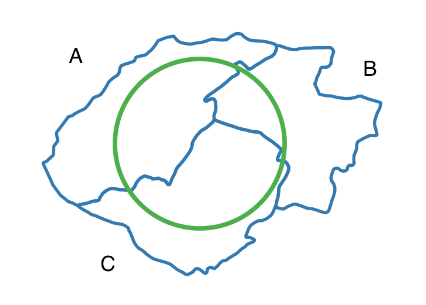
We don’t know how the population is distributed inside these municipalities. They are probably concentrated in cities somewhere, but, since we don’t know where they are, our best guess is to assume that the population is evenly distributed in the municipality (i.e. every point inside the municipality has the same population density).
Population is an extensive property (it grows with area), so we can subset it (a region inside the municipality will always have a smaller population than the whole municipality), and also aggregate it by summing.
In this case, we’d calculate the population inside each part of the circle that intersects with a municipality.
Default aggregation methods
In the Data Observatory, we suggest a default aggregation method for certain fields. However, some fields don’t have a clear best method, and some just can’t be aggregated. In these cases, we leave the agg_method field blank and let the user choose the method that best fits their needs.
Conclusion
In this guide you've seen how to use CARTOframes in conjunction with the Data Observatory to enrich a Starbucks dataset with a new population variable for the use case of revenue prediction analysis by:
- Choosing the total population variable from the Data Observatory catalog
- Calculating the sum of total population for each store
- Calculating the sum of total population around the walking areas of influence around each store
In addition, you were introduced to some more advanced concepts and further explanation of how the enrichment itself works.