DeepCube Use Case 3: Fire Hazard Forecasting in the Mediterranean
![]()
Notebook 2: Fire danger maps in Greece with Deep Learning models
This notebook shows how to load our pretrained models for Fire Danger prediction to perform inference on the published greece_wildfire_datacube or its cloud version.
For details about how our models were trained, have a look at our relevant paper "Deep Learning Methods for Daily Wildfire Danger Forecasting" available on arXiv, which is accepted to the workshop on Artificial Intelligence for Humanitarian Assistance and Disaster Response at the 35th Conference on Neural Information Processing Systems (NeurIPS 2021)

Initial Imports
We start by importing the libraries we need. Make sure to have them installed in your system.
import xarray as xr
import fsspec
import zarr

import numpy as np
import pandas as pd

import csv
import numpy as np
import matplotlib.pyplot as plt

import random
import os
from tqdm import tqdm
import gc
from pathlib import Path

import torchvision
import torch
from torch.utils.data import Dataset, DataLoader, TensorDataset
Access Datacube
Let's open the dataset with xarray
# uncomment the lines if you download the dataset locally
# !wget -O dataset_greece.nc https://zenodo.org/record/4943354/files/dataset_greece.nc?download=1
# ds = xr.open_dataset('./dataset_greece.nc')

# comment out the following two lines if you want to access the dataset locally
url = 'https://storage.de.cloud.ovh.net/v1/AUTH_84d6da8e37fe4bb5aea18902da8c1170/uc3/uc3cube.zarr'
ds = xr.open_zarr(fsspec.get_mapper(url), consolidated=True)
ds
<xarray.Dataset>
Dimensions:                  (time: 4314, x: 700, y: 562)
Coordinates:
    band                     int64 ...
    spatial_ref              (time) int64 dask.array<chunksize=(288,), meta=np.ndarray>
  * time                     (time) datetime64[ms] 2009-03-06 ... 2020-12-26
  * x                        (x) float64 19.86 19.87 19.89 ... 28.16 28.17 28.18
  * y                        (y) float64 41.62 41.61 41.59 ... 34.96 34.95 34.94
Data variables: (12/58)
    1 km 16 days EVI         (time, y, x) float64 dask.array<chunksize=(288, 50, 50), meta=np.ndarray>
    1 km 16 days NDVI        (time, y, x) float64 dask.array<chunksize=(288, 50, 50), meta=np.ndarray>
    1 km 16 days VI Quality  (time, y, x) float64 dask.array<chunksize=(288, 50, 50), meta=np.ndarray>
    ET_500m                  (time, y, x) float64 dask.array<chunksize=(288, 50, 50), meta=np.ndarray>
    ET_QC_500m               (time, y, x) float64 dask.array<chunksize=(288, 50, 50), meta=np.ndarray>
    FparExtra_QC             (time, y, x) float64 dask.array<chunksize=(288, 50, 50), meta=np.ndarray>
    ...                       ...
    population_density_2020  (y, x) float32 dask.array<chunksize=(50, 50), meta=np.ndarray>
    roads_density_2020       (y, x) float64 dask.array<chunksize=(50, 50), meta=np.ndarray>
    slope_max                (y, x) float32 dask.array<chunksize=(50, 50), meta=np.ndarray>
    slope_mean               (y, x) float32 dask.array<chunksize=(50, 50), meta=np.ndarray>
    slope_min                (y, x) float32 dask.array<chunksize=(50, 50), meta=np.ndarray>
slope_std (y, x) float32 dask.array<chunksize=(50, 50), meta=np.ndarray>- time: 4314
- x: 700
- y: 562
- band()int64...
- name :
- band
array(0)
- spatial_ref(time)int64dask.array<chunksize=(288,), meta=np.ndarray>
- GeoTransform :
- 19.852811908702186 0.0002341811352383137 0.0 41.6273340924137 0.0 -0.00023418113523831377
- crs_wkt :
- GEOGCS["WGS 84",DATUM["WGS_1984",SPHEROID["WGS 84",6378137,298.257223563,AUTHORITY["EPSG","7030"]],AUTHORITY["EPSG","6326"]],PRIMEM["Greenwich",0,AUTHORITY["EPSG","8901"]],UNIT["degree",0.0174532925199433,AUTHORITY["EPSG","9122"]],AXIS["Latitude",NORTH],AXIS["Longitude",EAST],AUTHORITY["EPSG","4326"]]
- geographic_crs_name :
- WGS 84
- grid_mapping_name :
- latitude_longitude
- inverse_flattening :
- 298.257223563
- longitude_of_prime_meridian :
- 0.0
- name :
- spatial_ref
- prime_meridian_name :
- Greenwich
- reference_ellipsoid_name :
- WGS 84
- semi_major_axis :
- 6378137.0
- semi_minor_axis :
- 6356752.314245179
- spatial_ref :
- GEOGCS["WGS 84",DATUM["WGS_1984",SPHEROID["WGS 84",6378137,298.257223563,AUTHORITY["EPSG","7030"]],AUTHORITY["EPSG","6326"]],PRIMEM["Greenwich",0,AUTHORITY["EPSG","8901"]],UNIT["degree",0.0174532925199433,AUTHORITY["EPSG","9122"]],AXIS["Latitude",NORTH],AXIS["Longitude",EAST],AUTHORITY["EPSG","4326"]]
Array Chunk Bytes 33.70 kiB 2.25 kiB Shape (4314,) (288,) Count 16 Tasks 15 Chunks Type int64 numpy.ndarray - time(time)datetime64[ms]2009-03-06 ... 2020-12-26
array(['2009-03-06T00:00:00.000', '2009-03-07T00:00:00.000', '2009-03-08T00:00:00.000', ..., '2020-12-24T00:00:00.000', '2020-12-25T00:00:00.000', '2020-12-26T00:00:00.000'], dtype='datetime64[ms]') - x(x)float6419.86 19.87 19.89 ... 28.17 28.18
array([19.862915, 19.874819, 19.886723, ..., 28.16 , 28.171904, 28.183808])
- y(y)float6441.62 41.61 41.59 ... 34.95 34.94
array([41.617206, 41.605302, 41.593398, ..., 34.962873, 34.950969, 34.939065])
- 1 km 16 days EVI(time, y, x)float64dask.array<chunksize=(288, 50, 50), meta=np.ndarray>
- long_name :
- 1 km 16 days EVI
- name :
- 1 km 16 days EVI
- units :
- EVI
Array Chunk Bytes 12.64 GiB 5.49 MiB Shape (4314, 562, 700) (288, 50, 50) Count 2521 Tasks 2520 Chunks Type float64 numpy.ndarray - 1 km 16 days NDVI(time, y, x)float64dask.array<chunksize=(288, 50, 50), meta=np.ndarray>
- long_name :
- 1 km 16 days NDVI
- name :
- 1 km 16 days NDVI
- units :
- NDVI
Array Chunk Bytes 12.64 GiB 5.49 MiB Shape (4314, 562, 700) (288, 50, 50) Count 2521 Tasks 2520 Chunks Type float64 numpy.ndarray - 1 km 16 days VI Quality(time, y, x)float64dask.array<chunksize=(288, 50, 50), meta=np.ndarray>
- long_name :
- 1 km 16 days VI Quality
- name :
- 1 km 16 days VI Quality
- units :
- bit field
Array Chunk Bytes 12.64 GiB 5.49 MiB Shape (4314, 562, 700) (288, 50, 50) Count 2521 Tasks 2520 Chunks Type float64 numpy.ndarray - ET_500m(time, y, x)float64dask.array<chunksize=(288, 50, 50), meta=np.ndarray>
- long_name :
- MODIS Gridded 500m 8-day Composite Evapotranspiration (ET)
- name :
- ET_500m
- units :
- kg/m^2/8day
Array Chunk Bytes 12.64 GiB 5.49 MiB Shape (4314, 562, 700) (288, 50, 50) Count 2521 Tasks 2520 Chunks Type float64 numpy.ndarray - ET_QC_500m(time, y, x)float64dask.array<chunksize=(288, 50, 50), meta=np.ndarray>
- long_name :
- ET_QC_500m
- name :
- ET_QC_500m
- units :
- none
Array Chunk Bytes 12.64 GiB 5.49 MiB Shape (4314, 562, 700) (288, 50, 50) Count 2521 Tasks 2520 Chunks Type float64 numpy.ndarray - FparExtra_QC(time, y, x)float64dask.array<chunksize=(288, 50, 50), meta=np.ndarray>
- long_name :
- MOD15A2H MODIS/Terra+Aqua pass-through QC for FPAR and LAI (8-day composite)
- name :
- FparExtra_QC
- units :
- class-flag
Array Chunk Bytes 12.64 GiB 5.49 MiB Shape (4314, 562, 700) (288, 50, 50) Count 2521 Tasks 2520 Chunks Type float64 numpy.ndarray - FparLai_QC(time, y, x)float64dask.array<chunksize=(288, 50, 50), meta=np.ndarray>
- long_name :
- MOD15A2H MODIS/Terra+Aqua QC for FPAR and LAI (8-day composite)
- name :
- FparLai_QC
- units :
- class-flag
Array Chunk Bytes 12.64 GiB 5.49 MiB Shape (4314, 562, 700) (288, 50, 50) Count 2521 Tasks 2520 Chunks Type float64 numpy.ndarray - FparStdDev_500m(time, y, x)float64dask.array<chunksize=(288, 50, 50), meta=np.ndarray>
- long_name :
- MOD15A2H MODIS/Terra Gridded 500M Standard Deviation FPAR (8-day composite)
- name :
- FparStdDev_500m
- units :
- Percent
Array Chunk Bytes 12.64 GiB 5.49 MiB Shape (4314, 562, 700) (288, 50, 50) Count 2521 Tasks 2520 Chunks Type float64 numpy.ndarray - Fpar_500m(time, y, x)float64dask.array<chunksize=(288, 50, 50), meta=np.ndarray>
- long_name :
- MOD15A2H MODIS/Terra Gridded 500M FPAR (8-day composite)
- name :
- Fpar_500m
- units :
- Percent
Array Chunk Bytes 12.64 GiB 5.49 MiB Shape (4314, 562, 700) (288, 50, 50) Count 2521 Tasks 2520 Chunks Type float64 numpy.ndarray - LE_500m(time, y, x)float64dask.array<chunksize=(288, 50, 50), meta=np.ndarray>
- long_name :
- MODIS Gridded 500m 8-day Composite latent heat flux (LE)
- name :
- LE_500m
- units :
- J/m^2/day
Array Chunk Bytes 12.64 GiB 5.49 MiB Shape (4314, 562, 700) (288, 50, 50) Count 2521 Tasks 2520 Chunks Type float64 numpy.ndarray - LST_Day_1km(time, y, x)float64dask.array<chunksize=(288, 50, 50), meta=np.ndarray>
- long_name :
- Daily daytime 1km grid Land-surface Temperature
- name :
- LST_Day_1km
- units :
- K
Array Chunk Bytes 12.64 GiB 5.49 MiB Shape (4314, 562, 700) (288, 50, 50) Count 2521 Tasks 2520 Chunks Type float64 numpy.ndarray - LST_Night_1km(time, y, x)float64dask.array<chunksize=(288, 50, 50), meta=np.ndarray>
- long_name :
- Daily nighttime 1km grid Land-surface Temperature
- name :
- LST_Night_1km
- units :
- K
Array Chunk Bytes 12.64 GiB 5.49 MiB Shape (4314, 562, 700) (288, 50, 50) Count 2521 Tasks 2520 Chunks Type float64 numpy.ndarray - LaiStdDev_500m(time, y, x)float64dask.array<chunksize=(288, 50, 50), meta=np.ndarray>
- long_name :
- MOD15A2H MODIS/Terra Gridded 500M Standard Deviation Leaf Area Index (8-day composite)
- name :
- LaiStdDev_500m
- units :
- m^2/m^2
Array Chunk Bytes 12.64 GiB 5.49 MiB Shape (4314, 562, 700) (288, 50, 50) Count 2521 Tasks 2520 Chunks Type float64 numpy.ndarray - Lai_500m(time, y, x)float64dask.array<chunksize=(288, 50, 50), meta=np.ndarray>
- long_name :
- MOD15A2H MODIS/Terra Gridded 500M Leaf Area Index LAI (8-day composite)
- name :
- Lai_500m
- units :
- m^2/m^2
Array Chunk Bytes 12.64 GiB 5.49 MiB Shape (4314, 562, 700) (288, 50, 50) Count 2521 Tasks 2520 Chunks Type float64 numpy.ndarray - PET_500m(time, y, x)float64dask.array<chunksize=(288, 50, 50), meta=np.ndarray>
- long_name :
- MODIS Gridded 500m 8-day Composite potential Evapotranspiration (ET)
- name :
- PET_500m
- units :
- kg/m^2/8day
Array Chunk Bytes 12.64 GiB 5.49 MiB Shape (4314, 562, 700) (288, 50, 50) Count 2521 Tasks 2520 Chunks Type float64 numpy.ndarray - PLE_500m(time, y, x)float64dask.array<chunksize=(288, 50, 50), meta=np.ndarray>
- long_name :
- MODIS Gridded 500m 8-day Composite potential latent heat flux (LE)
- name :
- PLE_500m
- units :
- J/m^2/day
Array Chunk Bytes 12.64 GiB 5.49 MiB Shape (4314, 562, 700) (288, 50, 50) Count 2521 Tasks 2520 Chunks Type float64 numpy.ndarray - QC_Day(time, y, x)float64dask.array<chunksize=(288, 50, 50), meta=np.ndarray>
- long_name :
- Quality control for daytime LST and emissivity
- name :
- QC_Day
Array Chunk Bytes 12.64 GiB 5.49 MiB Shape (4314, 562, 700) (288, 50, 50) Count 2521 Tasks 2520 Chunks Type float64 numpy.ndarray - QC_Night(time, y, x)float64dask.array<chunksize=(288, 50, 50), meta=np.ndarray>
- long_name :
- Quality control for nighttime LST and emissivity
- name :
- QC_Night
Array Chunk Bytes 12.64 GiB 5.49 MiB Shape (4314, 562, 700) (288, 50, 50) Count 2521 Tasks 2520 Chunks Type float64 numpy.ndarray - aspect_max(y, x)float32dask.array<chunksize=(50, 50), meta=np.ndarray>
- name :
- aspect_max
Array Chunk Bytes 1.50 MiB 9.77 kiB Shape (562, 700) (50, 50) Count 169 Tasks 168 Chunks Type float32 numpy.ndarray - aspect_mean(y, x)float32dask.array<chunksize=(50, 50), meta=np.ndarray>
- name :
- aspect_mean
Array Chunk Bytes 1.50 MiB 9.77 kiB Shape (562, 700) (50, 50) Count 169 Tasks 168 Chunks Type float32 numpy.ndarray - aspect_min(y, x)float32dask.array<chunksize=(50, 50), meta=np.ndarray>
- name :
- aspect_min
Array Chunk Bytes 1.50 MiB 9.77 kiB Shape (562, 700) (50, 50) Count 169 Tasks 168 Chunks Type float32 numpy.ndarray - aspect_std(y, x)float32dask.array<chunksize=(50, 50), meta=np.ndarray>
- name :
- aspect_std
Array Chunk Bytes 1.50 MiB 9.77 kiB Shape (562, 700) (50, 50) Count 169 Tasks 168 Chunks Type float32 numpy.ndarray - burned_areas(time, y, x)float64dask.array<chunksize=(288, 50, 50), meta=np.ndarray>
- name :
- burned_areas
Array Chunk Bytes 12.64 GiB 5.49 MiB Shape (4314, 562, 700) (288, 50, 50) Count 2521 Tasks 2520 Chunks Type float64 numpy.ndarray - clc_2006(y, x)float32dask.array<chunksize=(50, 50), meta=np.ndarray>
- RepresentationType :
- THEMATIC
- STATISTICS_COVARIANCES :
- 134.7975361912512
- STATISTICS_MAXIMUM :
- 48
- STATISTICS_MEAN :
- 25.790668746788
- STATISTICS_MINIMUM :
- 1
- STATISTICS_SKIPFACTORX :
- 1
- STATISTICS_SKIPFACTORY :
- 1
- STATISTICS_STDDEV :
- 11.610234114403
- name :
- clc_2006
Array Chunk Bytes 1.50 MiB 9.77 kiB Shape (562, 700) (50, 50) Count 169 Tasks 168 Chunks Type float32 numpy.ndarray - clc_2012(y, x)float32dask.array<chunksize=(50, 50), meta=np.ndarray>
- RepresentationType :
- THEMATIC
- STATISTICS_COVARIANCES :
- 135.8886173847565
- STATISTICS_MAXIMUM :
- 48
- STATISTICS_MEAN :
- 25.733156200754
- STATISTICS_MINIMUM :
- 1
- STATISTICS_SKIPFACTORX :
- 1
- STATISTICS_SKIPFACTORY :
- 1
- STATISTICS_STDDEV :
- 11.65712732129
- name :
- clc_2012
Array Chunk Bytes 1.50 MiB 9.77 kiB Shape (562, 700) (50, 50) Count 169 Tasks 168 Chunks Type float32 numpy.ndarray - clc_2018(y, x)float32dask.array<chunksize=(50, 50), meta=np.ndarray>
- RepresentationType :
- THEMATIC
- STATISTICS_COVARIANCES :
- 136.429646247598
- STATISTICS_MAXIMUM :
- 48
- STATISTICS_MEAN :
- 25.753373398066
- STATISTICS_MINIMUM :
- 1
- STATISTICS_SKIPFACTORX :
- 1
- STATISTICS_SKIPFACTORY :
- 1
- STATISTICS_STDDEV :
- 11.680310194836
- name :
- clc_2018
Array Chunk Bytes 1.50 MiB 9.77 kiB Shape (562, 700) (50, 50) Count 169 Tasks 168 Chunks Type float32 numpy.ndarray - dem_max(y, x)float32dask.array<chunksize=(50, 50), meta=np.ndarray>
- BandName :
- Band_1
- RepresentationType :
- ATHEMATIC
- STATISTICS_COVARIANCES :
- 170299.0228961734
- STATISTICS_MAXIMUM :
- 2905.8544921875
- STATISTICS_MEAN :
- 430.74131537734
- STATISTICS_MINIMUM :
- -36.388916015625
- STATISTICS_SKIPFACTORX :
- 1
- STATISTICS_SKIPFACTORY :
- 1
- STATISTICS_STDDEV :
- 412.67302176926
- long_name :
- Band_1
- name :
- dem_max
Array Chunk Bytes 1.50 MiB 9.77 kiB Shape (562, 700) (50, 50) Count 169 Tasks 168 Chunks Type float32 numpy.ndarray - dem_mean(y, x)float32dask.array<chunksize=(50, 50), meta=np.ndarray>
- BandName :
- Band_1
- RepresentationType :
- ATHEMATIC
- STATISTICS_COVARIANCES :
- 170299.0228961734
- STATISTICS_MAXIMUM :
- 2905.8544921875
- STATISTICS_MEAN :
- 430.74131537734
- STATISTICS_MINIMUM :
- -36.388916015625
- STATISTICS_SKIPFACTORX :
- 1
- STATISTICS_SKIPFACTORY :
- 1
- STATISTICS_STDDEV :
- 412.67302176926
- long_name :
- Band_1
- name :
- dem_mean
Array Chunk Bytes 1.50 MiB 9.77 kiB Shape (562, 700) (50, 50) Count 169 Tasks 168 Chunks Type float32 numpy.ndarray - dem_min(y, x)float32dask.array<chunksize=(50, 50), meta=np.ndarray>
- BandName :
- Band_1
- RepresentationType :
- ATHEMATIC
- STATISTICS_COVARIANCES :
- 170299.0228961734
- STATISTICS_MAXIMUM :
- 2905.8544921875
- STATISTICS_MEAN :
- 430.74131537734
- STATISTICS_MINIMUM :
- -36.388916015625
- STATISTICS_SKIPFACTORX :
- 1
- STATISTICS_SKIPFACTORY :
- 1
- STATISTICS_STDDEV :
- 412.67302176926
- long_name :
- Band_1
- name :
- dem_min
Array Chunk Bytes 1.50 MiB 9.77 kiB Shape (562, 700) (50, 50) Count 169 Tasks 168 Chunks Type float32 numpy.ndarray - dem_std(y, x)float32dask.array<chunksize=(50, 50), meta=np.ndarray>
- BandName :
- Band_1
- RepresentationType :
- ATHEMATIC
- STATISTICS_COVARIANCES :
- 170299.0228961734
- STATISTICS_MAXIMUM :
- 2905.8544921875
- STATISTICS_MEAN :
- 430.74131537734
- STATISTICS_MINIMUM :
- -36.388916015625
- STATISTICS_SKIPFACTORX :
- 1
- STATISTICS_SKIPFACTORY :
- 1
- STATISTICS_STDDEV :
- 412.67302176926
- long_name :
- Band_1
- name :
- dem_std
Array Chunk Bytes 1.50 MiB 9.77 kiB Shape (562, 700) (50, 50) Count 169 Tasks 168 Chunks Type float32 numpy.ndarray - era5_max_t2m(time, y, x)float32dask.array<chunksize=(288, 50, 50), meta=np.ndarray>
- long_name :
- 2 metre temperature
- name :
- era5_max_t2m
- units :
- K
Array Chunk Bytes 6.32 GiB 2.75 MiB Shape (4314, 562, 700) (288, 50, 50) Count 2521 Tasks 2520 Chunks Type float32 numpy.ndarray - era5_max_tp(time, y, x)float32dask.array<chunksize=(288, 50, 50), meta=np.ndarray>
- long_name :
- Total precipitation
- name :
- era5_max_tp
- units :
- m
Array Chunk Bytes 6.32 GiB 2.75 MiB Shape (4314, 562, 700) (288, 50, 50) Count 2521 Tasks 2520 Chunks Type float32 numpy.ndarray - era5_max_u10(time, y, x)float32dask.array<chunksize=(288, 50, 50), meta=np.ndarray>
- long_name :
- 10 metre U wind component
- name :
- era5_max_u10
- units :
- m s**-1
Array Chunk Bytes 6.32 GiB 2.75 MiB Shape (4314, 562, 700) (288, 50, 50) Count 2521 Tasks 2520 Chunks Type float32 numpy.ndarray - era5_max_v10(time, y, x)float32dask.array<chunksize=(288, 50, 50), meta=np.ndarray>
- long_name :
- 10 metre V wind component
- name :
- era5_max_v10
- units :
- m s**-1
Array Chunk Bytes 6.32 GiB 2.75 MiB Shape (4314, 562, 700) (288, 50, 50) Count 2521 Tasks 2520 Chunks Type float32 numpy.ndarray - era5_min_t2m(time, y, x)float32dask.array<chunksize=(288, 50, 50), meta=np.ndarray>
- long_name :
- 2 metre temperature
- name :
- era5_min_t2m
- units :
- K
Array Chunk Bytes 6.32 GiB 2.75 MiB Shape (4314, 562, 700) (288, 50, 50) Count 2521 Tasks 2520 Chunks Type float32 numpy.ndarray - era5_min_tp(time, y, x)float32dask.array<chunksize=(288, 50, 50), meta=np.ndarray>
- long_name :
- Total precipitation
- name :
- era5_min_tp
- units :
- m
Array Chunk Bytes 6.32 GiB 2.75 MiB Shape (4314, 562, 700) (288, 50, 50) Count 2521 Tasks 2520 Chunks Type float32 numpy.ndarray - era5_min_u10(time, y, x)float32dask.array<chunksize=(288, 50, 50), meta=np.ndarray>
- long_name :
- 10 metre U wind component
- name :
- era5_min_u10
- units :
- m s**-1
Array Chunk Bytes 6.32 GiB 2.75 MiB Shape (4314, 562, 700) (288, 50, 50) Count 2521 Tasks 2520 Chunks Type float32 numpy.ndarray - era5_min_v10(time, y, x)float32dask.array<chunksize=(288, 50, 50), meta=np.ndarray>
- long_name :
- 10 metre V wind component
- name :
- era5_min_v10
- units :
- m s**-1
Array Chunk Bytes 6.32 GiB 2.75 MiB Shape (4314, 562, 700) (288, 50, 50) Count 2521 Tasks 2520 Chunks Type float32 numpy.ndarray - fwi(time, y, x)float32dask.array<chunksize=(288, 50, 50), meta=np.ndarray>
- name :
- fwi
- title :
- Fire Weather Index
- units :
- -
Array Chunk Bytes 6.32 GiB 2.75 MiB Shape (4314, 562, 700) (288, 50, 50) Count 2521 Tasks 2520 Chunks Type float32 numpy.ndarray - ignition_points(time, y, x)float64dask.array<chunksize=(288, 50, 50), meta=np.ndarray>
- name :
- ignition_points
Array Chunk Bytes 12.64 GiB 5.49 MiB Shape (4314, 562, 700) (288, 50, 50) Count 2521 Tasks 2520 Chunks Type float64 numpy.ndarray - number_of_fires(time)int64dask.array<chunksize=(288,), meta=np.ndarray>
- name :
- number_of_fires
Array Chunk Bytes 33.70 kiB 2.25 kiB Shape (4314,) (288,) Count 16 Tasks 15 Chunks Type int64 numpy.ndarray - population_density_2009(y, x)float32dask.array<chunksize=(50, 50), meta=np.ndarray>
- STATISTICS_MAXIMUM :
- 30021.15234375
- STATISTICS_MEAN :
- 82.238914394041
- STATISTICS_MINIMUM :
- 0
- STATISTICS_STDDEV :
- 671.48598504916
- name :
- population_density_2009
Array Chunk Bytes 1.50 MiB 9.77 kiB Shape (562, 700) (50, 50) Count 169 Tasks 168 Chunks Type float32 numpy.ndarray - population_density_2010(y, x)float32dask.array<chunksize=(50, 50), meta=np.ndarray>
- STATISTICS_MAXIMUM :
- 30363.30859375
- STATISTICS_MEAN :
- 82.147479667057
- STATISTICS_MINIMUM :
- 0
- STATISTICS_STDDEV :
- 671.88602769617
- name :
- population_density_2010
Array Chunk Bytes 1.50 MiB 9.77 kiB Shape (562, 700) (50, 50) Count 169 Tasks 168 Chunks Type float32 numpy.ndarray - population_density_2011(y, x)float32dask.array<chunksize=(50, 50), meta=np.ndarray>
- STATISTICS_MAXIMUM :
- 30233.619140625
- STATISTICS_MEAN :
- 82.027437460922
- STATISTICS_MINIMUM :
- 0
- STATISTICS_STDDEV :
- 670.9042302745
- name :
- population_density_2011
Array Chunk Bytes 1.50 MiB 9.77 kiB Shape (562, 700) (50, 50) Count 169 Tasks 168 Chunks Type float32 numpy.ndarray - population_density_2012(y, x)float32dask.array<chunksize=(50, 50), meta=np.ndarray>
- STATISTICS_MAXIMUM :
- 30224.205078125
- STATISTICS_MEAN :
- 82.107784707183
- STATISTICS_MINIMUM :
- 0
- STATISTICS_STDDEV :
- 690.0772575156
- name :
- population_density_2012
Array Chunk Bytes 1.50 MiB 9.77 kiB Shape (562, 700) (50, 50) Count 169 Tasks 168 Chunks Type float32 numpy.ndarray - population_density_2013(y, x)float32dask.array<chunksize=(50, 50), meta=np.ndarray>
- STATISTICS_MAXIMUM :
- 29517.470703125
- STATISTICS_MEAN :
- 81.931516848424
- STATISTICS_MINIMUM :
- 0
- STATISTICS_STDDEV :
- 687.19612524192
- name :
- population_density_2013
Array Chunk Bytes 1.50 MiB 9.77 kiB Shape (562, 700) (50, 50) Count 169 Tasks 168 Chunks Type float32 numpy.ndarray - population_density_2014(y, x)float32dask.array<chunksize=(50, 50), meta=np.ndarray>
- STATISTICS_MAXIMUM :
- 30178.935546875
- STATISTICS_MEAN :
- 81.840487639716
- STATISTICS_MINIMUM :
- 0
- STATISTICS_STDDEV :
- 686.75219541252
- name :
- population_density_2014
Array Chunk Bytes 1.50 MiB 9.77 kiB Shape (562, 700) (50, 50) Count 169 Tasks 168 Chunks Type float32 numpy.ndarray - population_density_2015(y, x)float32dask.array<chunksize=(50, 50), meta=np.ndarray>
- STATISTICS_MAXIMUM :
- 29919.798828125
- STATISTICS_MEAN :
- 81.714012872504
- STATISTICS_MINIMUM :
- 0
- STATISTICS_STDDEV :
- 684.62444513266
- name :
- population_density_2015
Array Chunk Bytes 1.50 MiB 9.77 kiB Shape (562, 700) (50, 50) Count 169 Tasks 168 Chunks Type float32 numpy.ndarray - population_density_2016(y, x)float32dask.array<chunksize=(50, 50), meta=np.ndarray>
- STATISTICS_MAXIMUM :
- 30245.38671875
- STATISTICS_MEAN :
- 81.694480644465
- STATISTICS_MINIMUM :
- 0
- STATISTICS_STDDEV :
- 687.63942943867
- name :
- population_density_2016
Array Chunk Bytes 1.50 MiB 9.77 kiB Shape (562, 700) (50, 50) Count 169 Tasks 168 Chunks Type float32 numpy.ndarray - population_density_2017(y, x)float32dask.array<chunksize=(50, 50), meta=np.ndarray>
- STATISTICS_MAXIMUM :
- 30296.751953125
- STATISTICS_MEAN :
- 81.73828589391
- STATISTICS_MINIMUM :
- 0
- STATISTICS_STDDEV :
- 687.54544893798
- name :
- population_density_2017
Array Chunk Bytes 1.50 MiB 9.77 kiB Shape (562, 700) (50, 50) Count 169 Tasks 168 Chunks Type float32 numpy.ndarray - population_density_2018(y, x)float32dask.array<chunksize=(50, 50), meta=np.ndarray>
- STATISTICS_MAXIMUM :
- 30178.298828125
- STATISTICS_MEAN :
- 81.510859548732
- STATISTICS_MINIMUM :
- 0
- STATISTICS_STDDEV :
- 685.82322299114
- name :
- population_density_2018
Array Chunk Bytes 1.50 MiB 9.77 kiB Shape (562, 700) (50, 50) Count 169 Tasks 168 Chunks Type float32 numpy.ndarray - population_density_2019(y, x)float32dask.array<chunksize=(50, 50), meta=np.ndarray>
- STATISTICS_MAXIMUM :
- 29704.583984375
- STATISTICS_MEAN :
- 81.406228331852
- STATISTICS_MINIMUM :
- 0
- STATISTICS_STDDEV :
- 682.22370306917
- name :
- population_density_2019
Array Chunk Bytes 1.50 MiB 9.77 kiB Shape (562, 700) (50, 50) Count 169 Tasks 168 Chunks Type float32 numpy.ndarray - population_density_2020(y, x)float32dask.array<chunksize=(50, 50), meta=np.ndarray>
- STATISTICS_MAXIMUM :
- 29829.5859375
- STATISTICS_MEAN :
- 81.333684900144
- STATISTICS_MINIMUM :
- 0
- STATISTICS_STDDEV :
- 681.53318412642
- name :
- population_density_2020
Array Chunk Bytes 1.50 MiB 9.77 kiB Shape (562, 700) (50, 50) Count 169 Tasks 168 Chunks Type float32 numpy.ndarray - roads_density_2020(y, x)float64dask.array<chunksize=(50, 50), meta=np.ndarray>
- name :
- roads_density_2020
Array Chunk Bytes 3.00 MiB 19.53 kiB Shape (562, 700) (50, 50) Count 169 Tasks 168 Chunks Type float64 numpy.ndarray - slope_max(y, x)float32dask.array<chunksize=(50, 50), meta=np.ndarray>
- name :
- slope_max
Array Chunk Bytes 1.50 MiB 9.77 kiB Shape (562, 700) (50, 50) Count 169 Tasks 168 Chunks Type float32 numpy.ndarray - slope_mean(y, x)float32dask.array<chunksize=(50, 50), meta=np.ndarray>
- name :
- slope_mean
Array Chunk Bytes 1.50 MiB 9.77 kiB Shape (562, 700) (50, 50) Count 169 Tasks 168 Chunks Type float32 numpy.ndarray - slope_min(y, x)float32dask.array<chunksize=(50, 50), meta=np.ndarray>
- name :
- slope_min
Array Chunk Bytes 1.50 MiB 9.77 kiB Shape (562, 700) (50, 50) Count 169 Tasks 168 Chunks Type float32 numpy.ndarray - slope_std(y, x)float32dask.array<chunksize=(50, 50), meta=np.ndarray>
- name :
- slope_std
Array Chunk Bytes 1.50 MiB 9.77 kiB Shape (562, 700) (50, 50) Count 169 Tasks 168 Chunks Type float32 numpy.ndarray
We see that the dataset has x,y and time dimensions.
More specifically it contains 4314 days (from 06/03/2009 to 06/12/2020) of 700x562 rasters
Dynamic variables like the burned_areas have all three dimensions, while static variables like clc_2012 misses the temporal component and only has x, y dimensions.
Method Description
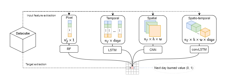
From the datacube, we extract four different datasets that are used to train four different models. For a given pixel (i.e., a cell representing a 1 km x 1 km square region) and a given day, we extract input-target pairs for 4 different modeling modalities:
- First, the pixel dataset, where we extract the input attributes and their last 10-day average (only for the dynamic input attributes). This is used to train a Random Forest (RF) model (is not shown in this notebook).
- Second, the temporal dataset, where we extract the last 10-day time-series of the input attributes. This is used to train an Long Short-Term Memory (LSTM) model.
- Third, the spatial dataset, where we extract 25km x 25km patches spatially centered around the given pixel. This is used to train a Convolutional Neural Network (CNN) model.
- Fourth, the spatio-temporal dataset, where we extract 25km x 25km x 10 days blocks centered spatially around the given pixel. This is used to train a convLSTM model.
Load pretrained models
Pytorch lightning checkpoints are on saved_models directory.
The code for the models is in the src directory.
from src.greece_fire_models import CNN_fire_model, LSTM_fire_model, ConvLSTM_fire_model
# these are the features that change in time
dynamic_features = ['Fpar_500m', 'Lai_500m', 'LST_Day_1km', 'LST_Night_1km', '1 km 16 days NDVI', '1 km 16 days EVI', 'era5_max_u10', 'era5_max_v10', 'era5_max_t2m', 'era5_max_tp', 'era5_min_u10', 'era5_min_v10', 'era5_min_t2m']
# these are the features that remain the same through time
static_features= ['dem_mean', 'aspect_mean', 'slope_mean', 'roads_density_2020', 'population_density']
# the settings that were used to train our best models
best_settings = {
    'lstm' : {'dynamic_features' : dynamic_features, 'static_features' : static_features , 'hidden_size' : 64,  'lstm_layers':1, 'attention':False},
    'cnn' : {'dynamic_features' : dynamic_features, 'static_features' : static_features , 'hidden_size' : 16},
    'convlstm' : {'dynamic_features' : dynamic_features, 'static_features' : static_features , 'hidden_size' : 16,  'lstm_layers':1},

}
model = 'lstm'
lstm = LSTM_fire_model(**best_settings[model]).load_from_checkpoint('saved_models/lstm.ckpt')
model = 'cnn'
cnn = CNN_fire_model(**best_settings[model]).load_from_checkpoint('saved_models/cnn.ckpt')
model = 'convlstm'
convlstm = ConvLSTM_fire_model(**best_settings[model]).load_from_checkpoint('saved_models/convlstm.ckpt')
Do inference
The models have been trained using data for the years 2009-2019. We will perform inference on two days of the test set (year 2020).
from src.greece_fire_dataset import FireDatasetWholeDay

def predict_map(day, pl_module, access_mode, problem_class, patch_size, lag, dynamic_features, static_features, nan_fill, batch_size):
    """
    This function returns the predictions of model (pl_module) for a given day.
    """
    dataset = FireDatasetWholeDay(ds, day, access_mode, problem_class, patch_size, lag,
                                  dynamic_features,
                                  static_features,
                                  nan_fill)
    len_x = dataset.len_x
    len_y = dataset.len_y
    pl_module.eval()
    num_iterations = max(1, len(dataset) // batch_size)
    dataloader = DataLoader(dataset, batch_size=batch_size, shuffle=False,
                            num_workers=num_workers, prefetch_factor=batch_size)
    outputs = []
    for i, (dynamic, static) in tqdm(enumerate(dataloader), total=num_iterations):

        if pl_module.on_gpu:
            inputs = inputs.cuda()
        logits = pl_module(inputs)
        preds_proba = torch.exp(logits)[:, 1]
        outputs.append(preds_proba.detach().cpu())
    outputs = torch.cat(outputs, dim=0)
    outputs = outputs.reshape(len_y, len_x)
    outputs = outputs.detach().cpu().numpy().squeeze()
    return outputs
# days for which to create fire danger maps
days = [4150, 4155]
patch_size = 25
lag = 10
# value used to fill nans
nan_fill = -1.0

acc_mod_bs = [('spatial', cnn, 4096, 'CNN'), ('temporal', lstm, 10196, 'LSTM'), ('spatiotemporal', convlstm, 512, 'ConvLSTM'), ]
problem_class='classification'
num_workers = 12

# these are used to mask out land cover classes that are not supposed to be dangerous for fire (sea, water bodies, urban areas)
clc = np.isin(ds['clc_2012'].values, list(range(12, 33)), invert=True)
pop_den = np.isnan(ds['population_density_2012'].values)
for day in days:
    gc.collect()
    day = int(day)
    print(day)
    # get a validation batch from the validation dat loader
    fig, ax = plt.subplots(1,4, figsize=(20,5))
    fig.suptitle('Fire danger for Greece on {}'.format(ds['time'][day].dt.strftime('%d/%m/%Y').values))
    subplot_number = 141
    for i, (access_mode, pl_module, batch_size, name) in enumerate(acc_mod_bs):
        if access_mode == 'spatial':
            lag = 0
        else:
            lag = 10
        if access_mode == 'temporal':
            patch_size = 0
        else:
            patch_size = 25
        outputs =  predict_map(day, pl_module, access_mode, problem_class, patch_size,
                               lag, dynamic_features, static_features, nan_fill, batch_size)
        outputs[clc] = 0
        outputs[pop_den] = 0
        plt.subplot(subplot_number), plt.imshow(outputs, vmin=0, vmax=1, cmap='Spectral_r')
        plt.title(name)
        subplot_number += 1
    fwi = ds.fwi[day].values
    fwi[clc] = 0
    fwi[pop_den] = 0
    plt.subplot(subplot_number), plt.imshow(fwi, vmin=0, vmax=50, cmap='Spectral_r')
    plt.title('FWI')
    plt.show()
4150
97it [04:18,  2.66s/it]
39it [05:21,  8.25s/it]
769it [06:18,  2.03it/s]

4155
97it [04:19,  2.67s/it]
39it [05:24,  8.33s/it]
769it [06:21,  2.02it/s]

We see that the danger maps created by the Deep Learning models follow closely, but offer a better resolution than the empirical Fire Weather Index that is widely used as an operational tool. This is quite an interesting result, considering that our models have been trained using the historical burned areas as target and do not have a direct notion of what Fire Danger is. This is quite a step forward in showing that fire danger can be learned in a data driven way and it is possible to leverage what DL models can learn from the complex interactions of the Fire Drivers.
Discussion
We see that the danger maps created by the Deep Learning models follow closely, but offer a better resolution than the empirical Fire Weather Index that is widely used as an operational tool. This is quite an interesting result, considering that our models have been trained using the historical burned areas as target and do not have a direct notion of what Fire Danger is. This is quite a step forward in showing that fire danger can be learned in a data driven way and it is possible to leverage what DL models can learn from the complex interactions of the Fire Drivers.
In this notebook, we saw how to load pytorch lighning pretrained Deep Learning modules and use them on inference to create fire danger maps. In a later notebook we'll use explainable AI methods to understand our models' predictions. Stay tuned!
Acknowledgements
Research funded by the EU H2020 project DeepCube ’Explainable AI pipelines for big Copernicus data’, grant agreement No 101004188.
Notebook Authors: Ioannis Prapas (https://github.com/iprapas), Spyros Kondylatos (https://github.com/skondylatos)