Python Programming
Our goal is to lay out a program that gets results. We will learn and discover!
This top-down learning is different. We will go directly to coding and start practicing. This will give us a context for connecting with deeper knowledge. It is iterative and we will improve with practice.
Our Workshop Google Doc has a code reference sheet
Core Concepts:
- loops
- functions
- conditionals
- exploratory data analysis
Session 1 Agenda:
- Syntax Sandbox
- Starting Our challenge
- Load Libraries
- Load and inspect data: functions, methods, and loops!
- Access parts of the dataframe and plot data!
- Your Challenge
Session 2 Agenda
- Use conditional if-elif-else statements to explore data based on value
- Data Visualizations with Seaborn
Session 3 Agenda
- Writing Functions
- Statistical Analysis
Syntax Sandbox 
# Hashtag denotes a comment
In Python, variable names:
- can include letters, digits, and underscores
- cannot start with a digit
- are case sensitive
This means that, for example:
weight0is a valid variable name, whereas0weightis notweightandWeightare different variables
# [1]:
weight_kg = 60
weight_lb = 2.2 * weight_kg
print(weight_lb, weight_kg)
132.0 60
Variables only change value when something is assigned to them.
If we make one cell in a spreadsheet depend on another, and update the latter, the former updates automatically. This does not happen in programming languages.
# [2]:
weight_kg = 70
print(weight_lb, weight_kg)
132.0 70
Data types are:
- integer numbers
- floating point numbers, and
- strings (text)
# [3]:
weight_kg = 60.3
type(weight_kg)
float
# [4]:
weight_kg = '60.3'
type(weight_kg)
str
Need help?
# [5]:
#help(print)
#?print
# [6]:
# Conversion tools are built in
#weight_lb = 2.2 * weight_kg
#weight_lb = 2.2 * float(weight_kg)
print(weight_lb)
132.0
- Basic data types in Python include integers, strings, and floating-point numbers.
- Use `variable = value` to assign a value to a variable in order to record it in memory.
- Use `print(something)` to display the value of something.
- Must convert numbers to strings or float and int when operating on them.
- Variables only change value when something is assigned to them.
Our Challenge: Analyze Amazon Top 50 Bestselling Books 📗
- Amazon.com is one of the largest online marketplace and many people around the world purchase products.
- In this notebook, we observe the data about top 50 bestselling books from 2009 to 2019 on Amazon.
- Amazon Top 50 Bestselling Books 2009 - 2019 (Kaggle.com)

1. Load libraries. 
Think of these as useful powerful toolboxes we are opening up on our workbench. Many additional libraries are available from the Python Package Index.
- numpy - adding support for large, multi-dimensional arrays and matrices, and mathematical functions for arrays.
- pandas - offers data structures and operations for manipulating numerical tables and time series.
- matplotlib - the most widely used scientific plotting library in Python.
- seaborn - for drawing attractive and informative statistical graphics.
# [7]:
import numpy as np
import pandas as pd

# Libraris for plotting
import matplotlib.pyplot as plt
import seaborn as sns

# Library for hypothesis testing
from scipy import stats

# Library for regression modeling
import statsmodels as sm
from statsmodels.formula.api import ols

# Library for latex
from IPython.display import Latex
2. Load data.
Loads a copy of the data into our environment. Unlike working with a spreadsheet, it does not affect the original file.
Read a Comma Separated Values (CSV) data file with pd.read_csv(). Need to read in a different file type?
- Argument is the name of the file to be read.
- Assign result to a variable to store the data that was read.
# [8]:
url = "https://raw.githubusercontent.com/DeisData/pystats/main/bestsellers_with_categories.csv"
books = pd.read_csv(url)
3. Inspect the data table 
There are lots of functions and methods we can apply to the dataframe to start inspecting it.
# [9]:
# Function to print a view of the data
print(books)
                                                  Name  \
0                        10-Day Green Smoothie Cleanse
1                                    11/22/63: A Novel
2              12 Rules for Life: An Antidote to Chaos
3                               1984 (Signet Classics)
4    5,000 Awesome Facts (About Everything!) (Natio...
..                                                 ...
545       Wrecking Ball (Diary of a Wimpy Kid Book 14)
546  You Are a Badass: How to Stop Doubting Your Gr...
547  You Are a Badass: How to Stop Doubting Your Gr...
548  You Are a Badass: How to Stop Doubting Your Gr...
549  You Are a Badass: How to Stop Doubting Your Gr...

                       Author  User Rating  Reviews  Price  Year        Genre
0                    JJ Smith          4.7    17350      8  2016  Non Fiction
1                Stephen King          4.6     2052     22  2011      Fiction
2          Jordan B. Peterson          4.7    18979     15  2018  Non Fiction
3               George Orwell          4.7    21424      6  2017      Fiction
4    National Geographic Kids          4.8     7665     12  2019  Non Fiction
..                        ...          ...      ...    ...   ...          ...
545               Jeff Kinney          4.9     9413      8  2019      Fiction
546               Jen Sincero          4.7    14331      8  2016  Non Fiction
547               Jen Sincero          4.7    14331      8  2017  Non Fiction
548               Jen Sincero          4.7    14331      8  2018  Non Fiction
549               Jen Sincero          4.7    14331      8  2019  Non Fiction

[550 rows x 7 columns]
# [10]:
# Method to view head of dataset
books.head()
| Name | Author | User Rating | Reviews | Price | Year | Genre | |
|---|---|---|---|---|---|---|---|
| 0 | 10-Day Green Smoothie Cleanse | JJ Smith | 4.7 | 17350 | 8 | 2016 | Non Fiction |
| 1 | 11/22/63: A Novel | Stephen King | 4.6 | 2052 | 22 | 2011 | Fiction |
| 2 | 12 Rules for Life: An Antidote to Chaos | Jordan B. Peterson | 4.7 | 18979 | 15 | 2018 | Non Fiction |
| 3 | 1984 (Signet Classics) | George Orwell | 4.7 | 21424 | 6 | 2017 | Fiction |
| 4 | 5,000 Awesome Facts (About Everything!) (Natio... | National Geographic Kids | 4.8 | 7665 | 12 | 2019 | Non Fiction |
# [11]:
# Method to see the tail end of the data
books.tail()
| Name | Author | User Rating | Reviews | Price | Year | Genre | |
|---|---|---|---|---|---|---|---|
| 545 | Wrecking Ball (Diary of a Wimpy Kid Book 14) | Jeff Kinney | 4.9 | 9413 | 8 | 2019 | Fiction |
| 546 | You Are a Badass: How to Stop Doubting Your Gr... | Jen Sincero | 4.7 | 14331 | 8 | 2016 | Non Fiction |
| 547 | You Are a Badass: How to Stop Doubting Your Gr... | Jen Sincero | 4.7 | 14331 | 8 | 2017 | Non Fiction |
| 548 | You Are a Badass: How to Stop Doubting Your Gr... | Jen Sincero | 4.7 | 14331 | 8 | 2018 | Non Fiction |
| 549 | You Are a Badass: How to Stop Doubting Your Gr... | Jen Sincero | 4.7 | 14331 | 8 | 2019 | Non Fiction |
# [12]:
# Use the DataFrame.info() method to find out more about a dataframe.
books.info()
<class 'pandas.core.frame.DataFrame'>
RangeIndex: 550 entries, 0 to 549
Data columns (total 7 columns):
 #   Column       Non-Null Count  Dtype
---  ------       --------------  -----
 0   Name         550 non-null    object
 1   Author       550 non-null    object
 2   User Rating  550 non-null    float64
 3   Reviews      550 non-null    int64
 4   Price        550 non-null    int64
 5   Year         550 non-null    int64
 6   Genre        550 non-null    object
dtypes: float64(1), int64(3), object(3)
memory usage: 30.2+ KB
# [13]:
# Get Dimensions (rows, columns)
books.shape
(550, 7)
# [14]:
# Get data types
books.dtypes
Name            object
Author          object
User Rating    float64
Reviews          int64
Price            int64
Year             int64
Genre           object
dtype: object
# [15]:
# Use DataFrame.describe() to get summary statistics about data.
books.describe()
| User Rating | Reviews | Price | Year | |
|---|---|---|---|---|
| count | 550.000000 | 550.000000 | 550.000000 | 550.000000 |
| mean | 4.618364 | 11953.281818 | 13.100000 | 2014.000000 |
| std | 0.226980 | 11731.132017 | 10.842262 | 3.165156 |
| min | 3.300000 | 37.000000 | 0.000000 | 2009.000000 |
| 25% | 4.500000 | 4058.000000 | 7.000000 | 2011.000000 |
| 50% | 4.700000 | 8580.000000 | 11.000000 | 2014.000000 |
| 75% | 4.800000 | 17253.250000 | 16.000000 | 2017.000000 |
| max | 4.900000 | 87841.000000 | 105.000000 | 2019.000000 |
# [16]:
# The DataFrame.columns variable stores information about the dataframe’s columns.
books.columns
Index(['Name', 'Author', 'User Rating', 'Reviews', 'Price', 'Year', 'Genre'], dtype='object')
Let's loop through them and make each column name follow variable name best practices.
# [17]:
# General format of a loop
for number in [2, 3, 5]:
    print(number*5)
10
15
25
# [18]:
# Application of a loop to fix DataFrame column names:

#1. Save DataFrame.column names to an object to be our loop collection
cols = books.columns

#2. Initialize some "empty storage" for corrected column names
new_column_names = []

#3. Loop through collection of column names
for col in cols:

    # strip beginning and ending spaces
    new_col = col.lstrip().rstrip()
    # make names lower case
    new_col = new_col.lower()
    # replace spaces with underscores
    new_col = new_col.replace(" ","_")

    print(new_col)

    # append each new column name to the new object of corrected names
    new_column_names.append(new_col)

# End of indention is end of loop body

# Assign new column names to DataFrame
books.columns = new_column_names
name
author
user_rating
reviews
price
year
genre
# [19]:
# Let's check the results!
books.head()
| name | author | user_rating | reviews | price | year | genre | |
|---|---|---|---|---|---|---|---|
| 0 | 10-Day Green Smoothie Cleanse | JJ Smith | 4.7 | 17350 | 8 | 2016 | Non Fiction |
| 1 | 11/22/63: A Novel | Stephen King | 4.6 | 2052 | 22 | 2011 | Fiction |
| 2 | 12 Rules for Life: An Antidote to Chaos | Jordan B. Peterson | 4.7 | 18979 | 15 | 2018 | Non Fiction |
| 3 | 1984 (Signet Classics) | George Orwell | 4.7 | 21424 | 6 | 2017 | Fiction |
| 4 | 5,000 Awesome Facts (About Everything!) (Natio... | National Geographic Kids | 4.8 | 7665 | 12 | 2019 | Non Fiction |
Tip: Need to loop through a set of files? Check out the glob library.
- Use the Pandas library to get basic statistics out of tabular data.
- Use `index_col` to specify that a column’s values should be used as row headings.
- Use `DataFrame.info` to find out more about a dataframe.
- The `DataFrame.columns` variable stores information about the dataframe’s columns.
- Use `DataFrame.T` to transpose a dataframe.
- Use `DataFrame.describe` to get summary statistics about data.
4. Access parts of the dataframe 
To access a value at the position [i,j] of a DataFrame, we have two options:
- Use
DataFrame.iloc[..., ...]to select values by their (entry) position. Position indexing starts at0. - Use
DataFrame.loc[..., ...]to select values by their (entry) label.
# [20]:
# Access all the rows : , and the 'User Rating' column with .loc method
books.loc[:, 'user_rating']
0      4.7
1      4.6
2      4.7
3      4.7
4      4.8
      ...
545    4.9
546    4.7
547    4.7
548    4.7
549    4.7
Name: user_rating, Length: 550, dtype: float64
# [21]:
# Access all the rows : , and the 'User Rating' column with .iloc method
books.iloc[:, 2]
0      4.7
1      4.6
2      4.7
3      4.7
4      4.8
      ...
545    4.9
546    4.7
547    4.7
548    4.7
549    4.7
Name: user_rating, Length: 550, dtype: float64
# [22]:
# or more simply, DataFrame.ColumnName
books.user_rating
0      4.7
1      4.6
2      4.7
3      4.7
4      4.8
      ...
545    4.9
546    4.7
547    4.7
548    4.7
549    4.7
Name: user_rating, Length: 550, dtype: float64
# [23]:
# Can we get a count of books per rating?
books.user_rating.groupby(books.user_rating).count()
user_rating
3.3      1
3.6      1
3.8      2
3.9      3
4.0     14
4.1      6
4.2      8
4.3     25
4.4     38
4.5     60
4.6    105
4.7    108
4.8    127
4.9     52
Name: user_rating, dtype: int64
Group By: split-apply-combine
Pandas vectorizing methods and grouping operations are features that provide users much flexibility to analyse their data.
# [24]:
# Number of reviews for each user rating level
books.reviews.groupby(books.user_rating).sum()
user_rating
3.3       9372
3.6      14982
3.8      94530
3.9      73998
4.0     243266
4.1     194305
4.2      34268
4.3     209072
4.4     267481
4.5     553867
4.6     972304
4.7    1475380
4.8    1757694
4.9     673786
Name: reviews, dtype: int64
# [25]:
#Let's visualize it!
nreviews = books.reviews.groupby(books.user_rating).sum()
# print(nreviews.columns)
# We have an error if we ask for columns of nreviews!
# Why? It is a 1-d "Series" array, not a dataframe
# [26]:
# These output is a series (a 1-D array.)  We need a DataFrame to plot
nreviews = books.reviews.groupby(books.user_rating).sum()
# Convert to dataframe
nreviews = nreviews.to_frame()

print(nreviews.columns)
nreviews.head()
# Notice user_rating is the label for the index of rows.
# We need to treat it as a column for plotting.
Index(['reviews'], dtype='object')
| reviews | |
|---|---|
| user_rating | |
| 3.3 | 9372 |
| 3.6 | 14982 |
| 3.8 | 94530 |
| 3.9 | 73998 |
| 4.0 | 243266 |
# [27]:
# Treat user_rating as a column, not the index.name of rows
#df.index.name = 'newhead'
nreviews.index.name = 'user_rating'

#df.reset_index(inplace=True)
nreviews.reset_index(inplace=True)

print(nreviews.columns)
nreviews.head()
Index(['user_rating', 'reviews'], dtype='object')
| user_rating | reviews | |
|---|---|---|
| 0 | 3.3 | 9372 |
| 1 | 3.6 | 14982 |
| 2 | 3.8 | 94530 |
| 3 | 3.9 | 73998 |
| 4 | 4.0 | 243266 |
# [28]:
# Finally - a plot with Seaborn!
p = sns.barplot(x=nreviews.user_rating , y= nreviews.reviews)
p.set_ylabel("Reviews")
p.set_xlabel("User Rating")
Text(0.5, 0, 'User Rating')

Use comparisons to select data based on value
# [29]:
# Let's get all the books with an above average user rating
books_hirated = books[books.user_rating > books.user_rating.mean()]
#print(books_hirated)
- Use DataFrame.iloc[..., ...] to select values by integer location.
- Use : on its own to mean all columns or all rows.
- Select multiple columns or rows using DataFrame.loc and a named slice.
- Result of slicing can be used in further operations.
- Use comparisons to select data based on value.
5. Post-Session 1 Challenge 
How much would it cost us to buy all the best books (user_rating == 4.9)? where == means "is equal to"
# [30]:
# Try here!  Make an object that is a data subset of the best books
best_books = books[books.user_rating == 4.9]
#print(best_books)
best_books.head()
| name | author | user_rating | reviews | price | year | genre | |
|---|---|---|---|---|---|---|---|
| 40 | Brown Bear, Brown Bear, What Do You See? | Bill Martin Jr. | 4.9 | 14344 | 5 | 2017 | Fiction |
| 41 | Brown Bear, Brown Bear, What Do You See? | Bill Martin Jr. | 4.9 | 14344 | 5 | 2019 | Fiction |
| 81 | Dog Man and Cat Kid: From the Creator of Capta... | Dav Pilkey | 4.9 | 5062 | 6 | 2018 | Fiction |
| 82 | Dog Man: A Tale of Two Kitties: From the Creat... | Dav Pilkey | 4.9 | 4786 | 8 | 2017 | Fiction |
| 83 | Dog Man: Brawl of the Wild: From the Creator o... | Dav Pilkey | 4.9 | 7235 | 4 | 2018 | Fiction |
- Write a loop to add up the cost of all the best books
# [31]:
# Try here!
# General format of a loop
# for number in [2, 3, 5]:
#     print(number*5)

# Initialize a sum variable, then add to it in a loop on the best book prices
total_price = 0
# Set up your loop:
prices = best_books.price
for cost in prices:
    total_price = total_price + cost
    # or, a shorter way:
    #total_price += cost
print(total_price)
535
- What is a way you can solve this without loops?
# [32]:
# Try here!
best_books.price.sum()
535
- Use
sns.lmplotto see whatpriceversususer_ratinglooks like for thebooksdataset. Seaborn Example
# [33]:
# Try here!
p = sns.lmplot(x = "user_rating" , y = "price", data = books)
#hue="genre", col="year", col_wrap=3)
p.savefig("price_v_userrating.png")

Session 2 
We will
- Review our challenge from last time
- use conditional if-elif-else statements to explore data based on value
- practice Data Visualizations

We would like to divide the "Popularity" of books into four stages.
| Popularity Level | Ratings |
|---|---|
| Extremely Popular | 4.8 or 4.9 |
| Very Popular | 4.5 ~ 4.7 |
| Fairly Popular | 4.0 ~ 4.4 |
| Popular | 3.3 ~ 3.9 |
Syntax Sandbox - Conditionals 
Conditionals are ways we can use values to decide what to do next in our analysis
# [34]:
# Making choices with conditional statements
num = 37
num > 100
False
We have operators for comparisons
>greater than<less than==is equal to!=is not equal>=is greater than or equal to<=is less than equal to
# [35]:
# if statement (conditional statement)
num = 37
if num > 100:
    print('greater')
else:
    print('is not greater')
print('done')
is not greater
done
# [36]:
# we can chain tests together using elif (else if)

num = -1
if num > 10:
    print(num, 'is positive and greater than ten')
elif num > 0:
    print(num, 'is positive and less than or equal to ten')
elif num == 0:
    print(num, 'is zero')
else:
    print(num, 'is negative')
-1 is negative
# [37]:

# Test multiple conditions in tests using "and" or "or"
x = 3
y = 5
if (x > 0 ) and (y >= 0):
    print('both parts are true')
else:
    print('at least one part false')
both parts are true
# [38]:

x = -3
y = -5
if (x < 0) or (y >= 0):
    print('at least one of these is true')
at least one of these is true
# [39]:

# Be aware of logic!
# What is the output of this code?
score = 77
if score > 60:
    grade = 'D'
elif score > 70:
    grade = 'C'
elif score > 80:
    grade = 'B'
else:
    grade = 'A'

print(grade)
D
1. Use conditionals to group the data 
We would like to use conditionals to divide the "Popularity" of books into four stages.
| Popularity Level | Ratings |
|---|---|
| Extremely Popular | 4.8 or 4.9 |
| Very Popular | 4.5 ~ 4.7 |
| Fairly Popular | 4.0 ~ 4.4 |
| Popular | 3.3 ~ 3.9 |
# [40]:
popularity = [0,0,0,0]
for i in books.user_rating:
    if i >= 4.8:
        popularity[0] += 1
    elif i >= 4.5:
        popularity[1] += 1
    elif i >= 4.0:
        popularity[2] += 1
    else:
        popularity[3] += 1
# [41]:
print(popularity)
[179, 273, 91, 7]
# [42]:
poplevels = ['Extremely Popular(4.8, 4.9)','Very Popular(4.4 - 4.7)','Fairly Popular(4.0 - 4.3)','Popular (- 3.9)']

# How do we make this into a dataframe so we can visualize it?
# Use pandas!
recats    = pd.DataFrame(
    {"x" : poplevels,
      "y": popularity
    })
print(recats)
                             x    y
0  Extremely Popular(4.8, 4.9)  179
1      Very Popular(4.4 - 4.7)  273
2    Fairly Popular(4.0 - 4.3)   91
3              Popular (- 3.9)    7
2. Visualize Relationships with Seaborn 
On Seaborn’s official website, they state:
If matplotlib “tries to make easy things easy and hard things possible”, seaborn makes a well-defined set of hard things easy too, including:
- Using default themes that are aesthetically pleasing.
- Setting custom color palettes.
- Making attractive statistical plots.
- Easily and flexibly displaying distributions.
- Visualizing information from matrices and DataFrames.
Here, Seaborn is our tool of choice for Exploratory Analysis.
Statistical analysis is a process of understanding how variables in a dataset relate to each other and how those relationships depend on other variables. Visualization can be a core component of this process because, when data are visualized properly, the human eye can see trends and patterns that indicate a relationship.
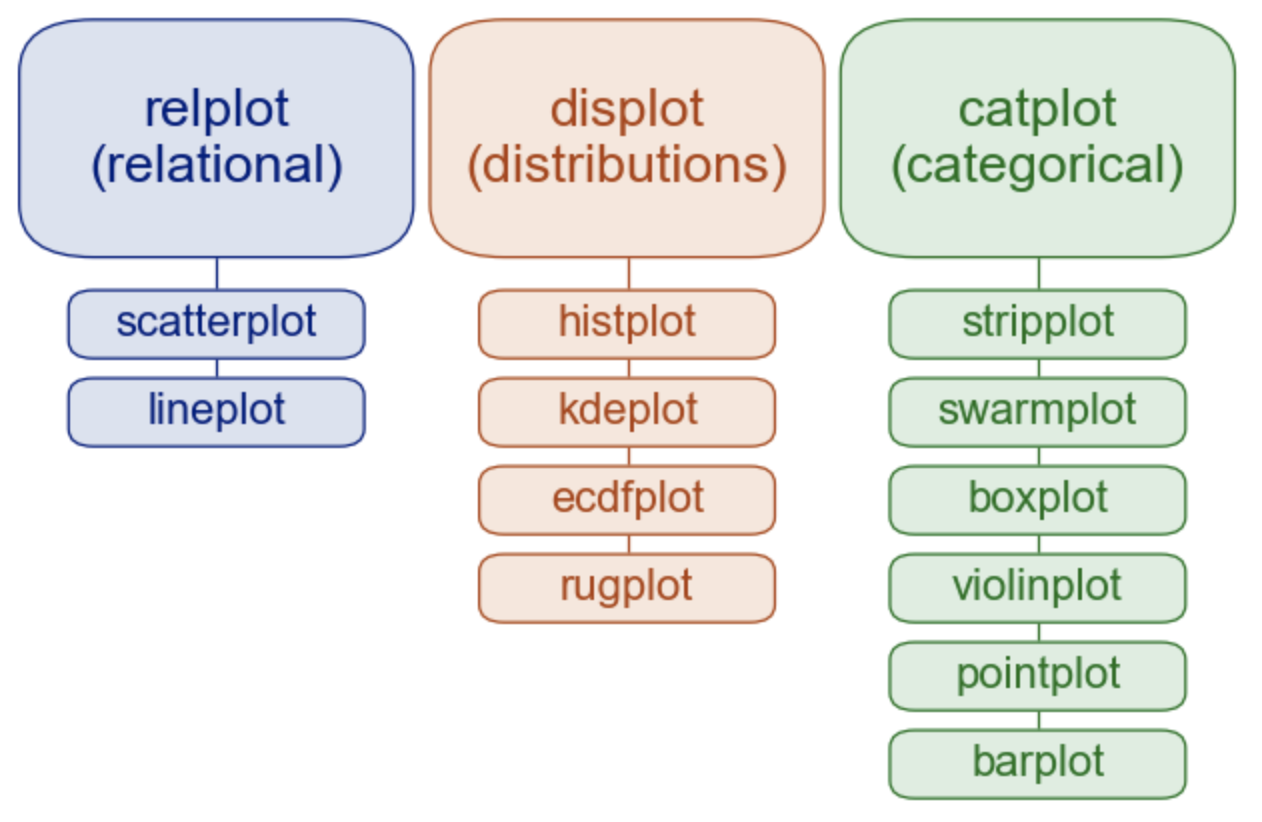
Overview of seaborn plotting functions
Most of your interactions with seaborn will happen through a set of plotting functions.
# [43]:
# Let's visualize the popularity category counts with a barplot!
fig = sns.catplot(kind="bar", data=recats, x=poplevels, y=popularity)

# We can use tools from matplotlib to make it look nicer
fig.set_xticklabels(rotation=30)
<seaborn.axisgrid.FacetGrid at 0x7f8dd37a2af0>

Data Exploration: Does the name 📖 of books affect User Rating?
- The name of books is very important, because readers get a first impression from it.
- Of course, the book which has short title is not always popular, and vice versa.
- However, the short title has the advantage of being simple and easy to understand, and the long title has that of giving readers an accurate understanding of what the book is like.
- Then, we try to find out the relationships between the length of name and rating.
# [44]:
# for loop for finding the name lengths
name_len = []
for i in books.name:
    name_len.append(len(i))
#print(name_len)
We want to put this with our data as a new column so we can make comparisons!
Search: how to append new column to a dataframe python pandas: Top result
# [45]:
# Using 'name_length' as the column name
# and equating it to the list
books['name_length'] = name_len

# Observe the result
#print(books)
Q: Does the name of books affect User Rating?
How should we compare two quantitative variables to see if there is correlation?
Let's look at the seaborn gallery
# [46]:
sns.scatterplot(x="name_length", y="user_rating",
                #hue="genre",
                data=books)
<AxesSubplot:xlabel='name_length', ylabel='user_rating'>

Can we look at all the quantitative data at once?
pairplot() combines joint and marginal views — but rather than focusing on a single relationship, it visualizes every pairwise combination of variables simultaneously:
# [47]:
sns.pairplot(data=books, hue="genre")
<seaborn.axisgrid.PairGrid at 0x7f8dd39a8b50>

Challenge 2
Question 1. Thinking through conditionals. Consider this code:
# [48]:
x = 4

if x > 5:
    print('A')
elif x == 5:
    print('B')
elif x < 5:
    print('C')
C
Which of the following would be printed if you were to run this code? Why did you pick this answer?
- A
- B
- C
- B and C
What is the answer if x = 5.0?
Question 2. Visually compare the User Rating versus Name Length for data with year==2019. Then, try to color-code the graph by genre using hue=?
# [49]:
# Try it!:

sns.scatterplot(x="name_length", y="user_rating",
                hue="genre",
                data=books[books.year==2019])
<AxesSubplot:xlabel='name_length', ylabel='user_rating'>

Break programs down into functions to make them easier to understand. Also enables re-use.
Define a function using def with a name, parameters, and a block of code.
# [50]
# Our first function!
def print_greeting():
    print('Hello!')
Defining a function does not run it.
# [51]
# Let's call our function!
print_greeting()
Hello!
Arguments in call are matched to parameters in definition.
# [52]
def print_date(year, month, day):
    joined = str(year) + '/' + str(month) + '/' + str(day)
    print(joined)
# [53]
print_date(1871, 3, 19)
1871/3/19
Or, we can name the arguments when we call the function, which allows us to specify them in any order:
# [54]
print_date(month=3, day=19, year=1871)
1871/3/19
Functions may return a result to their caller using return.
- Use
return ...to give a value back to the caller
# [55]
def temp_in_celsius(temp_f = 32):
    temp_c = (temp_f - 32 )* 5/9
    return temp_c
# [56]
# Call our function
temp_in_celsius()
0.0
Applying Functions to Data
Let's write a function that plots a subset of the data and saves it, but only if there are at least 10 rows of data
# [57]
# Defining the plotter function

def plotter(subset_data, fig_name):
    '''
    plotter returns a pairplot if there are at least 10 rows of data
    arguments are the dataframe subset_data and
    a figure name to output fig_name

    >>>plotter(author_data, 'authorname.png')
    '''

    # Get dimensions
    dimensions = subset_data.shape

    # Only make a plot if they've had more than 10 books on best-seller list
    # Conditional statement
    if dimensions[0] > 10:
        print(fig_name)
        fig = sns.pairplot(data=subset_data, hue="genre")
        fig.savefig(fig_name)
# [58]
help(plotter)
Help on function plotter in module __main__:

plotter(subset_data, fig_name)
    plotter returns a pairplot if there are at least 10 rows of data
    arguments are the dataframe subset_data and
    a figure name to output fig_name

    >>>plotter(author_data, 'authorname.png')
# [59]
# Now make use of this plotting function when we loop through authors
authors = books.author.unique()
#print(authors)
for author_name in authors:
    # Make a subset dataframe of the author's work
    authors_books = books[books.author==author_name]
    #authors_books.head()
    fig_name = author_name
    fig_name = fig_name.replace(" ","_")
    fig_name = fig_name.replace(".","")
    fig_name = fig_name +'.png'
    #print(fig_name)
    plotter(authors_books, fig_name)
Jeff_Kinney.png
Suzanne_Collins.png
Rick_Riordan.png
Gary_Chapman.png


# [60]
# Now make use of this plotting function when we loop through years
years = books.year.unique()

for year in years:
    # Make a subset dataframe of the author's work
    year_books = books[books.year==year]
    fig_name = 'year'+ str(year) + '.png'
    plotter(year_books, fig_name)
# [61]
# Extra Curious: Find books that were named on the list all more than 5 years
names = books.name.unique()

for title in names:
    if books[books.name==title].name.count() > 5:
        print(title)
Jesus Calling: Enjoying Peace in His Presence (with Scripture References)
Oh, the Places You'll Go!
Publication Manual of the American Psychological Association, 6th Edition
StrengthsFinder 2.0
The 7 Habits of Highly Effective People: Powerful Lessons in Personal Change
The Four Agreements: A Practical Guide to Personal Freedom (A Toltec Wisdom Book)
The Very Hungry Caterpillar
Hypothesis testing: Making statistical comparisons
For simple statistical tests, we will
use scipy.stats sub-module of scipy
1-sample t-test: testing the value of a population mean
scipy.stats.ttest_1samp tests if the population mean of data is
likely to be equal to a given value (technically if observations are
drawn from a Gaussian distributions of given population mean). It returns
the T statistic,
and the p-value.
Q: Is the mean of fiction book ratings different from the mean of all book ratings?
# [62]
# fiction books
fiction_books = books[books.genre=="Fiction"]

# mean of all book ratings
mean_rating = books.user_rating.mean()

# 1 sample t-test
stats.ttest_1samp(fiction_books.user_rating, mean_rating)
Ttest_1sampResult(statistic=1.7512207694305664, pvalue=0.08119072296558243)
With a p-value of $0.08$ we reject the hypothesis that the mean of fiction book ratings is significantly different from rating of all books at $\alpha=0.05$
2-sample t-test: testing for difference across populations
Let's do a 2-sample t-test
with scipy.stats.ttest_ind
Q: Is the name average length different between fiction and non-fiction books?
# [63]
fiction_names    = books[books.genre=="Fiction"].name_length
nonfiction_names = books[books.genre=="Non Fiction"].name_length
stats.ttest_ind(fiction_names, nonfiction_names)
Ttest_indResult(statistic=-10.164870067874736, pvalue=2.3627775756785156e-22)
With a p-value of $10^{-22}$ we reject the hypothesis that the mean name lengths of fiction and non-ficton books are equal.
Aside: Paired tests: repeated measurements on the same individuals
Paired tests are used if there are are links between observations: for example, if two variables are measured on the same individuals.
Thus the variance due to inter-subject variability is confounding, and can be removed, using a "paired test", or repeated measures test
# [64]
# We're not using it now, but the repeated measures 2-sample t-test is:
# stats.ttest_rel(variable1, variable2)
T-tests assume Gaussian errors. Non-parametric tests like Wilcoxon signed-rank test, that relaxes
this assumption. The corresponding test in the non paired case is the Mann–Whitney U test,
scipy.stats.mannwhitneyu.
# [65]
# Here, we use the Mann-Whitney test because we have
# different sample sizes of fiction and nonfiction books
# stats.wilcoxon(fiction_names, nonfiction_names)

stats.mannwhitneyu(fiction_names, nonfiction_names)
MannwhitneyuResult(statistic=20050.5, pvalue=8.482007241093608e-21)
Conclusion: we find that the data does support the hypothesis that fiction and non-fiction best-sellers have different name lengths
Linear models, multiple factors, and analysis of variance
We saw how easy it is to fit a simple linear regression in seaborn.
# [66]
# A simple linear regression
p = sns.lmplot(x = "user_rating" , y = "price", data = books)

Given two set of observations, x and y, we want to test the
hypothesis that y is a linear function of x. In other terms:
$y = x * \beta + \alpha + \epsilon$
where $\epsilon$ is observation noise.
We will use the statsmodels module to:
Fit a linear model. We will use the simplest strategy, ordinary least squares.
Test that the coefficient $\beta$ is non zero.
# [67]
# Then we specify an OLS model and fit it:
# Format:
# model = ols("y ~ x", data).fit()

p = sns.lmplot(x = "user_rating" , y = "price", data = books)

model = ols("price ~ user_rating", books).fit()


# We can inspect the various statistics derived from the fit::
print(model.summary())
                            OLS Regression Results
==============================================================================
Dep. Variable:                  price   R-squared:                       0.018
Model:                            OLS   Adj. R-squared:                  0.016
Method:                 Least Squares   F-statistic:                     9.881
Date:                Thu, 05 Aug 2021   Prob (F-statistic):            0.00176
Time:                        10:21:17   Log-Likelihood:                -2085.9
No. Observations:                 550   AIC:                             4176.
Df Residuals:                     548   BIC:                             4184.
Df Model:                           1
Covariance Type:            nonrobust
===============================================================================
                  coef    std err          t      P>|t|      [0.025      0.975]
-------------------------------------------------------------------------------
Intercept      42.4598      9.351      4.541      0.000      24.091      60.829
user_rating    -6.3572      2.022     -3.143      0.002     -10.330      -2.385
==============================================================================
Omnibus:                      476.250   Durbin-Watson:                   1.162
Prob(Omnibus):                  0.000   Jarque-Bera (JB):            12921.774
Skew:                           3.726   Prob(JB):                         0.00
Kurtosis:                      25.546   Cond. No.                         98.7
==============================================================================

Notes:
[1] Standard Errors assume that the covariance matrix of the errors is correctly specified.
Analysis of variance ANOVA
The ANOVA test has important assumptions that must be satisfied in order for the associated p-value to be valid.
The samples are independent. KS Test
Each sample is from a normally distributed population. Bartlett Test
The population standard deviations of the groups are all equal. This property is known as homoscedasticity.
If these assumptions are not true for a given set of data, it may still be possible to use the Kruskal-Wallis H-test (scipy.stats.kruskal) or the Alexander-Govern test (scipy.stats.alexandergovern) although with some loss of power.
# [68]
# Are the samples normally distributed?
sns.histplot(fiction_names)
stats.kstest(fiction_names,'norm')
KstestResult(statistic=0.9999999990134123, pvalue=0.0)

# [69]
sns.histplot(nonfiction_names)
stats.kstest(nonfiction_names,'norm')
KstestResult(statistic=0.9999683287581669, pvalue=0.0)

We reject the hypothesis that name lengths are normally distributed. This fails the assumption for ANOVA.
# [70]
# Are the standard deviations equal?
stats.bartlett(nonfiction_names, fiction_names)
BartlettResult(statistic=13.306986320333143, pvalue=0.00026441902180892425)
Reject the hypothesis that the non-fiction and fiction name lengths have equal variance. ANOVA assumptions are not met.
# [71]
# If ANOVA assumptions were met . . .
stats.f_oneway(nonfiction_names, fiction_names)
F_onewayResult(statistic=103.3245834967757, pvalue=2.3627775756782743e-22)
Since ANOVA assumptions were not met, we can consider a non-parametric test. The Kruskal-Wallis H-test tests the null hypothesis that the population median of all of the groups are equal.
# [72]
stats.kruskal(nonfiction_names, fiction_names)
KruskalResult(statistic=86.12153726045305, pvalue=1.6920990992638142e-20)
Reject the hypothesis that median name lengths are equal.
Challenge 3
Question 1: Earlier, we defined a function temp_in_celsius() that takes as an argument the temperature in Farhenheit, and applies a conversion calculation to Celsius.
Your first challenge, apply the function to a dataset measure_f of temperatures (in F).
# [73]
# Challenge: Apply our function to data
measure_f = [31, 2, -12, 40, 51, 37, 80]

# Try it here!
Question 2: Is there a relationship between name length and price? Consider:
- A t-test
- A linear regression fit
- A visual
# [74]
# Try it!
Key Points
Hypothesis testing and p-values give you the significance of an effect / difference.
Regressions enable you to express rich links in your data.
Visualizing your data and fitting simple models give insight into the data.
Resources 
- This workshop follows the guideance of Software Carpentry Lessons: Programming with Python
- Our dataset is Amazon Top 50 Bestselling Books 2009 - 2019 from Kaggle.com
- Request 1-1 consultations with Brandeis Data Services
- Take time with tutorials at Kaggle.com
- Brandeis LinkedIn Learning portal
- Stackoverflow
- Statsmodels User Guide
- Think stats book
- Pandas Cheat Sheet
- Pandas Getting Started Tutorials
- Data Visualization: Python Graph Gallery
- Seaborn example gallery
- Seaborn user guide and tutorial
- Anaconda documentation
Other Python Libraries
- SciPy is widely used in scientific and technical computing: optimization, linear algebra, integration, interpolation, special functions, FFT, signal and image processing, ODE solvers and other tasks
- Scikit-learn features various classification, regression and clustering algorithms including support vector machines, logistic regression, naive Bayes, random forests, gradient boosting, k-means and DBSCAN
- Mlpy is a Python machine learning library built on top of NumPy/SciPy
- NLTK The Natural Language Toolkit
Example solution to Session 3 Challenge 1
# Question 1 Example Solution

# Challenge: Apply our function to data
measure_f = [31, 2, -12, 40, 51, 37, 80]

# initialize storage
measure_c = []

# Use a for loop!
for tempf in measurements:
    measure_c.append(temp_in_celsius(tempf))

print(measure_c)
[-0.5555555555555556, -16.666666666666668, -24.444444444444443, 4.444444444444445, 10.555555555555555, 2.7777777777777777, 26.666666666666668]