Plans for this workshop
We're meeting today and tomorrow 1:30 - 3:00 pm
| Day 1 | Day 2 |
|---|---|
| Why Python for Data Science? | Data visualization |
| A Python Primer | Statistical modeling |
| Pandas for data munging | Machine learning |
Scope
Obviously we are going to cover each topic at a high level, given time constraints. I intend to give you a taste for what is possible
There are much more detailed resources available as Jupyter notebooks.
| Topic | Notebook |
|---|---|
| Python primer | 00_python_primer |
| Numpy and the data science stack (not covered) | 01_python_tools_ds |
| Pandas for data munging | 02_python_pandas |
| Data visualization | 03_python_vis |
| Statistical modeling | 04_python_stat |
| Machine learning | 05_python_learning |
Running notebooks on Binder
Binder is a free service that allows Python resources to be run on the web from Github repositories.
Why Python for Data Science?
Who is a data scientist?
One definition

Unclear definition
- Statistician
- Computer scientist
- Database engineer
- Software engineer
- Data engineer
- Mathematician
Some of the best ones I know are
neurobiologists and physicists
A broad umbrella
Anyone who wants to work with data to solve problems within particular domains
What it involves
What it involves
Managing and cleaning data
Interest in exploring relationships between things, informed by domain knowledge
Statistical know-how
Computational skills
Tools
We're here for the tools
The main two tools are
- Python (https://www.python.org)
- R (https://www.r-project.org)
There is a perpetual flame war between the two camps
That is not important
Why Python?
Pros
Very popular general purpose programming language
Strong ecosystem through packages (over 230K projects)
Succint syntax
Reasonably fast while also relatively easy to program
- Computational time vs Developer time
Self-documenting
Easier to integrate into production pipelines that already use Python
- Web frameworks (Django, Flask, ...)
- Workflow managers (Luigi, ...)
Increasingly strong Data Science Stack
Cons
- Not a rich-enough ecosystem for some purposes
- More computer science-y, less statistical
- Poorer frameworks for display and dissemination of information
These are areas where R tends to shine.
Python Data Science stack
Contributed packages over past 30 years
- To emulate Matlab
- Numpy
- Scipy
- Matplotlib
- To emulate Maple
- Sympy
- To add statistics/data science
- Pandas
- Various data visualization packages
- seaborn
- plotly
- Many more user-contributed packages
- The basic philosophy has been to concentrate on a few monolithic comprehensive packages
- statsmodels (Statistics)
- scikit-learn (Machine Learning)
- pillow (Image analysis)
- nltk (Natural Language Processing)
- tensorflow & PyTorch (Deep learning)
- PyMC3 (Bayesian learning)
Python as glue

- The
rpy2Python package is not developed on Windows - The
reticulateR package actually works quite well
- Data I/O
- We can read data from a variety of formats into Python
- Some proprietary
- R, SAS, Stata, SQL, Parquet, JSON
- We can read data from a variety of formats into Python
- There are ways of running R, SAS, others from within Python
- The Jupyter sub-ecosystem allows the same interface for many languages
- R, SAS, Julia, Haskell, Javascript
A Python Primer
Python is a popular, general purpose scripting language. The TIOBE index ranks Python as the third most popular programming language after C and Java, while this recent article in IEEE Computer Society says
"Python can be used for web and desktop applications, GUI-based desktop applications, machine learning, data science, and network servers. The programming language enjoys immense community support and offers several open-source libraries, frameworks, and modules that make application development a cakewalk." (Belani, 2020)
Python is a modular language
Python is not a monolithic language but is comprised of
- a base programming language
- numerous modules or libraries that add functionality to the language.
Python is a scripting language
Using Python requires typing!!
- You write code in Python
- that is then interpreted by the Python interpreter
- to make the computer implement your instructions.
Your code is like a recipe that you write for the computer.
Python is a high-level language in that the code is English-like and human-readable and understandable, which reduces the time needed for a person to create the recipe.
It is a language in that it has nouns (variables or objects), verbs (functions) and a structure or grammar that allows the programmer to write recipes for different functionalities.
Scripting can be frustrating in the beginning. You will find that the code you wrote doesn't work "for some reason", though it looks like you wrote it fine. The first things I look for, in order, are
One thing that is important to note in Python: case is important!. If we have two objects named data and Data, they will refer to different things.
- Did I spell all the variables and functions correctly
- Did I close all the brackets I have opened
- Did I finish all the quotes I started, and paired single- and double-quotes
- Did I already import the right module for the function I'm trying to use.
- Do I have the right indentations in my code.
These may not make sense right now, but as we go into Python, I hope you will remember these to help debug your code.
An example
Let's consider the following piece of Python code:
# set a splitting point
split_point = 3

# make two empty lists
lower = []; upper = []

# Split numbers from 0 to 9 into two groups,
# one lower or equal to the split point and
# one higher than the split point

for i in range(10):  # count from 0 to 9
    if i <= split_point:
        lower.append(i)
    else:
        upper.append(i)

print("lower:", lower)
print("upper:", upper)
lower: [0, 1, 2, 3]
upper: [4, 5, 6, 7, 8, 9]
First note that any line (or part of a line) starting with # is a comment in Python and is ignored by the interpreter. This makes it possible for us to write substantial text to remind us what each piece of our code does
The first piece of code that the Python interpreter actually reads is
split_point = 3
This takes the number 3 and stores it in the variable split_point. Variables are just names where some Python object is stored. It really works as an address to some particular part of your computer's memory, telling the Python interpreter to look for the value stored at that particular part of memory. Variable names allow your code to be human-readable since it allows you to write expressive names to remind yourself what you are storing. The rules of variable names are:
- Variable names must start with a letter or underscore
- The rest of the name can have letters, numbers or underscores
- Names are case-sensitive
The next piece of code initializes two lists, named lower and upper.
lower = []; upper = []
The semi-colon tells Python that, even though written on the same line, a particular instruction ends at the semi-colon, then another piece of instruction is written.
Lists are a catch-all data structure that can store different kinds of things, In this case we'll use them to store numbers.
for i in range(10):  # count from 0 to 9
    if i <= split_point
        lower.append(i)
    else:
        upper.append(i)
This is a for-loop.
- State with the numbers 0-9 (this is achieved in
range(10)) - Loop through each number, naming it
ieach time- Computer programs allow you to over-write a variable with a new value
- If the number currently stored in
iis less than or equal to the value ofsplit_point, i.e., 3 then add it to the listlower. Otherwise add it to the listupper
for i in range(10):  # count from 0 to 9
    if i <= split_point:
        lower.append(i)
    else:
        upper.append(i)
Note the indentation in the code. This is not by accident. Python understands the extent of a particular block of code within a for-loop (or within a if statement) using the indentations.
In this segment there are 3 code blocks:
- The for-loop as a whole (1st indentation)
- The
ifstatement testing if the number is less than or equal to the split point, telling Python what to do if the test is true - The
elsestatement stating what to do if the test in theifstatement is false
The last bit of code prints out the results
print("lower:", lower)
print("upper:", upper)
The print statement adds some text, and then prints out a representation of the object stored in the variable being printed. In this example, this is a list, and is printed as
lower: [0, 1, 2, 3]
upper: [4, 5, 6, 7, 8, 9]
We will expand on these concepts in the next few sections.
Some general rules on Python syntax
- Comments are marked by
# - A statement is terminated by the end of a line, or by a
;. - Indentation specifies blocks of code within particular structures. Whitespace at the beginning of lines matters. Typically you want to have 2 or 4 spaces to specify indentation, not a tab (\t) character. This can be set up in your IDE.
- Whitespace within lines does not matter, so you can use spaces liberally to make your code more readable
- Parentheses (
()) are for grouping pieces of code or for calling functions.
There are several conventions about code styling including the one in PEP8 (PEP = Python Enhancement Proposal) and one proposed by Google. We will typically be using lower case names, with words separated by underscores, in this workshop, basically following PEP8. Other conventions are of course allowed as long as they are within the basic rules stated above.
Data types
Numbers
- Floats (decimal numbers) :
float - Integers :
int
| Operation | Result |
|---|---|
| x + y | The sum of x and y |
| x - y | The difference of x and y |
| x * y | The product of x and y |
| x / y | The quotient of x and y |
| - x | The negative of x |
| abs(x) | The absolute value of x |
| x ** y | x raised to the power y |
| int(x) | Convert a number to integer |
| float(x) | Convert a number to floating point |
x = 3; y = 5

(2*x) -  (5 * y**2)
-119
Strings
first_name = 'Abhijit'
last_name = "Dasgupta"

'jit' in last_name
False
String operations
first_name + last_name

first_name*3

"gup" in last_name
Truthiness
Truthiness means evaluating the truth of a statement. This typically results in a Boolean object, which can take values True and False, but Python has several equivalent representations. The following values are considered the same as False:
None,False, zero (0,0L,0.0), any empty sequence ([],'',()), and a few others
All other values are considered True. Usually we'll denote truth by True and the number 1.
| Operation | Result |
|---|---|
| x < y | x is strictly less than y |
| x <= y | x is less than or equal to y |
| x == y | x equals y (note, it's 2 = signs) |
| x != y | x is not equal to y |
| x > y | x is strictly greater than y |
| x >= y | x is greater or equal to y |
We can chain these comparisons using Boolean operations
| Operation | Result |
|---|---|
| x | y | Either x is true or y is true or both |
| x & y | Both x and y are true |
| not x | if x is true, then false, and vice versa |
x = 5

(x < 3) | (x <= 7)
True
Variables are like individual ingredients in your recipe. It's mis en place or setting the table for any operations (functions) we want to do to them.
- Variables are like nouns,
- which will be acted on by verbs (functions).
In the next section we'll look at collections of variables. These collections are important in that it allows us to organize our variables with some structure.
Data structures
- Lists (
[]) - Tuples (
()) - Dictionaries or dicts (
{})
Lists are baskets that can contain different kinds of things. They are ordered, so that there is a first element, and a second element, and a last element, in order. However, the kinds of things in a single list doesn't have to be the same type.
Tuples are basically like lists, except that they are immutable, i.e., once they are created, individual values can't be changed. They are also ordered, so there is a first element, a second element and so on.
Dictionaries are unordered key-value pairs, which are very fast for looking up things. They work almost like hash tables. Dictionaries will be very useful to us as we progress towards the PyData stack. Elements need to be referred to by key, not by position.
test_list = ["apple", 3, True, "Harvey", 48205]
test_tuple = ("apple", 3, True, "Harvey", 48205)

test_list[0]
'apple'
| index | 0 | 1 | 2 | 3 | 4 |
| element | 'apple' | 3 | True | 'Harvey' | 48205 |
| counting backwards | -5 | -4 | -3 | -2 | -1 |
contact = {
    "first_name": "Abhijit",
    "last_name": "Dasgupta",
    "Age": 48,
    "address": "124 Main St",
    "Employed": True,
}
contact['first_name']
contact['address']
contact.keys()
contact.values()
Operations
Loops
pseudocode
Start with a list of datasets, one for each state
for each state
    compute and store fraction of votes that are Republican
    compute and store fraction of votes that are Democratic
for i in range(len(test_list)):
    print(test_list[i])
for u in test_list:
    print(u)
test_list2 = [1, 2, 3, 4, 5, 6, 7, 8, 9, 10]
mysum = 0
for u in test_list2:
    mysum = mysum + u
print(mysum)
enumerate automatically creates both the index and the value for each element of a list.
L = [0, 2, 4, 6, 8]
for i, val in enumerate(L):
    print(i, val)
0 0
1 2
2 4
3 6
4 8
zip puts multiple lists together and creates a composite iterator. You can have any number of iterators in zip, and the length of the result is determined by the length of the shortest iterator.
first = ["Han", "Luke", "Leia", "Anakin"]
last = ["Solo", "Skywalker", "Skywaker", "Skywalker"]
types = ['light','light','light','light/dark/light']

for val1, val2, val3 in zip(first, last, types):
    print(val1, val2, ' : ', val3)
Han Solo  :  light
Luke Skywalker  :  light
Leia Skywaker  :  light
Anakin Skywalker  :  light/dark/light
List comprehensions
test_list2 = [1,2,3,4,5,6]

squares = [u**2 for u in test_list2]
squares
Conditional evaluation
pseudocode
if Condition 1 is true then
    do Recipe 1
else if (elif) Condition 2 is true then
  do Recipe 2
else
  do Recipe 3
x = [-2, -1, 0, 1, 2, 3, 4, 5, 6, 7, 8, 9, 10]
y = []  # an empty list

for u in x:
    if u < 0:
        y.append("Negative")
    elif u % 2 == 1:  # what is remainder when dividing by 2
        y.append("Odd")
    else:
        y.append("Even")

print(y)
['Negative', 'Negative', 'Even', 'Odd', 'Even', 'Odd', 'Even', 'Odd', 'Even', 'Odd', 'Even', 'Odd', 'Even']
Functions
def my_mean(x):
    y = 0
    for u in x:
        y += u
    y = y / len(x)
    return y
A Python function must start with the keyword def followed by the name of the function, the arguments within parentheses, and then a colon. The actual code for the function is indented, just like in for-loops and if-elif-else structures. It ends with a return function which specifies the output of the function.
def my_mean(x):
    """
  A function to compute the mean of a list of numbers.

  INPUTS:
  x : a list containing numbers

  OUTPUT:
  The arithmetic mean of the list of numbers
  """
    y = 0
    for u in x:
        y = y + u
    y = y / len(x)
    return y
help(my_mean)
Help on function my_mean in module __main__:

my_mean(x)
    A function to compute the mean of a list of numbers.

    INPUTS:
    x : a list containing numbers

    OUTPUT:
    The arithmetic mean of the list of numbers
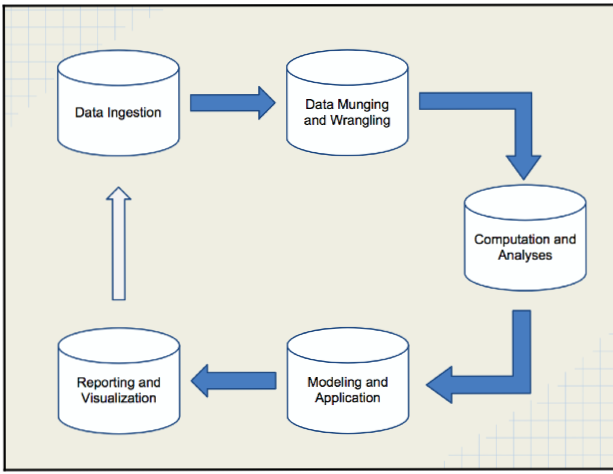
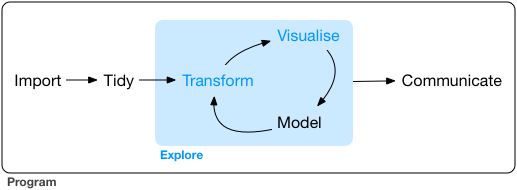
Pandas (Python Data Analysis)
- Data ingestion
- Data cleaning and transformation
- Data can be passed on to modeling and visualization packages
Activating packages for use
- Use the
importcommand - Maybe provide an alias for the package
import numpy as np
import pandas as pd
Data import
| Format type | Description | reader | writer |
|---|---|---|---|
| text | CSV | read_csv | to_csv |
| Excel | read_excel | to_excel | |
| text | JSON | read_json | to_json |
| binary | Feather | read_feather | to_feather |
| binary | SAS | read_sas | |
| SQL | SQL | read_sql | to_sql |
mtcars = pd.read_csv('data/mtcars.csv')
One of the big differences between a spreadsheet program and a programming language from the data science perspective is that you have to load data into the programming language. It's not "just there" like Excel. This is a good thing, since it allows the common functionality of the programming language to work across multiple data sets, and also keeps the original data set pristine. Excel users can run into problems and corrupt their data if they are not careful.
Exploring data
Creating a DataFrame
rng = np.random.RandomState(25)
d2 = pd.DataFrame(rng.normal(0,1, (4, 5)),
                  columns = ['A','B','C','D','E'],
                  index = ['a','b','c','d'])
d2
| A | B | C | D | E | |
|---|---|---|---|---|---|
| a | 0.228273 | 1.026890 | -0.839585 | -0.591182 | -0.956888 |
| b | -0.222326 | -0.619915 | 1.837905 | -2.053231 | 0.868583 |
| c | -0.920734 | -0.232312 | 2.152957 | -1.334661 | 0.076380 |
| d | -1.246089 | 1.202272 | -1.049942 | 1.056610 | -0.419678 |
A DataFrame has (mutable)
- An
index(row names) - A
column(column names)‘
d2.columns
d2.index
Index(['a', 'b', 'c', 'd'], dtype='object')
df = pd.DataFrame({
    'A':3.,
    'B':rng.random_sample(5),
    'C': pd.Timestamp('20200512'),
    'D': np.array([6] * 5),
    'E': pd.Categorical(['yes','no','no','yes','no']),
    'F': 'NIH'})
df
| A | B | C | D | E | F | |
|---|---|---|---|---|---|---|
| 0 | 3.0 | 0.481343 | 2020-05-12 | 6 | yes | NIH |
| 1 | 3.0 | 0.516502 | 2020-05-12 | 6 | no | NIH |
| 2 | 3.0 | 0.383048 | 2020-05-12 | 6 | no | NIH |
| 3 | 3.0 | 0.997541 | 2020-05-12 | 6 | yes | NIH |
| 4 | 3.0 | 0.514244 | 2020-05-12 | 6 | no | NIH |
You can also use a dict to create a DataFrame. If elements aren't of the same size, errors will be thrown, unless it is a single element. Then it will be repeated.
Slicing and dicing a DataFrame
df['B']
df.B
0    0.481343
1    0.516502
2    0.383048
3    0.997541
4    0.514244
Name: B, dtype: float64
There are two extractor functions in pandas:
locextracts by label (index label, column label, slice of labels, etc.ilocextracts by index (integers, slice objects, etc.
df.loc[1:3, 'C']
1   2020-05-12
2   2020-05-12
3   2020-05-12
Name: C, dtype: datetime64[ns]
You can also extract rows by condition (filter)
df = pd.DataFrame(np.random.randn(5, 3), index = ['a','c','e', 'f','g'], columns = ['one','two','three']) # pre-specify index and column names
df['four'] = 20 # add a column named "four", which will all be 20
df['five'] = df['one'] > 0
df
| one | two | three | four | five | |
|---|---|---|---|---|---|
| a | -0.847315 | 0.663926 | 0.182211 | 20 | False |
| c | 1.682927 | -0.056388 | 0.244149 | 20 | True |
| e | 0.185502 | 0.554072 | -0.739743 | 20 | True |
| f | -0.151335 | -0.172999 | -0.656354 | 20 | False |
| g | 0.672965 | -0.680025 | -0.065153 | 20 | True |
df[(df.one > 1) & (df.three < 0)]

df.query('(one > 1) & (three > 0)')
| one | two | three | four | five | |
|---|---|---|---|---|---|
| c | 1.682927 | -0.056388 | 0.244149 | 20 | True |
Replacing values
#df2.replace(0, -9) # replace 0 with -9

df.replace({'one': {5: 500}, 'three':{0:-9, 8:800}})
| one | two | three | four | five | |
|---|---|---|---|---|---|
| a | -0.847315 | 0.663926 | 0.182211 | 20 | False |
| c | 1.682927 | -0.056388 | 0.244149 | 20 | True |
| e | 0.185502 | 0.554072 | -0.739743 | 20 | True |
| f | -0.151335 | -0.172999 | -0.656354 | 20 | False |
| g | 0.672965 | -0.680025 | -0.065153 | 20 | True |
Joins
There are basically four kinds of joins:
| pandas | R | SQL | Description |
|---|---|---|---|
| left | left_join | left outer | keep all rows on left |
| right | right_join | right outer | keep all rows on right |
| outer | outer_join | full outer | keep all rows from both |
| inner | inner_join | inner | keep only rows with common keys |
Joins

survey = pd.read_csv('data/survey_survey.csv')
visited = pd.read_csv('data/survey_visited.csv')
pd.merge(survey, visited, left_on = 'taken', right_on = 'ident', how = 'left')
# survey.merge(visited, left_on = 'taken', right_on = 'ident', how = 'left')
| taken | person | quant | reading | ident | site | dated | |
|---|---|---|---|---|---|---|---|
| 0 | 619 | dyer | rad | 9.82 | 619 | DR-1 | 1927-02-08 |
| 1 | 619 | dyer | sal | 0.13 | 619 | DR-1 | 1927-02-08 |
| 2 | 622 | dyer | rad | 7.80 | 622 | DR-1 | 1927-02-10 |
| 3 | 622 | dyer | sal | 0.09 | 622 | DR-1 | 1927-02-10 |
| 4 | 734 | pb | rad | 8.41 | 734 | DR-3 | 1939-01-07 |
| 5 | 734 | lake | sal | 0.05 | 734 | DR-3 | 1939-01-07 |
| 6 | 734 | pb | temp | -21.50 | 734 | DR-3 | 1939-01-07 |
| 7 | 735 | pb | rad | 7.22 | 735 | DR-3 | 1930-01-12 |
| 8 | 735 | NaN | sal | 0.06 | 735 | DR-3 | 1930-01-12 |
| 9 | 735 | NaN | temp | -26.00 | 735 | DR-3 | 1930-01-12 |
| 10 | 751 | pb | rad | 4.35 | 751 | DR-3 | 1930-02-26 |
| 11 | 751 | pb | temp | -18.50 | 751 | DR-3 | 1930-02-26 |
| 12 | 751 | lake | sal | 0.10 | 751 | DR-3 | 1930-02-26 |
| 13 | 752 | lake | rad | 2.19 | 752 | DR-3 | NaN |
| 14 | 752 | lake | sal | 0.09 | 752 | DR-3 | NaN |
| 15 | 752 | lake | temp | -16.00 | 752 | DR-3 | NaN |
| 16 | 752 | roe | sal | 41.60 | 752 | DR-3 | NaN |
| 17 | 837 | lake | rad | 1.46 | 837 | MSK-4 | 1932-01-14 |
| 18 | 837 | lake | sal | 0.21 | 837 | MSK-4 | 1932-01-14 |
| 19 | 837 | roe | sal | 22.50 | 837 | MSK-4 | 1932-01-14 |
| 20 | 844 | roe | rad | 11.25 | 844 | DR-1 | 1932-03-22 |
Here, the left dataset is survey and the right one is visited.
Since we're doing a left join, we keed all the rows from survey and add columns from visited, matching on the common key, called "taken" in one dataset and "ident" in the other.
Note that the rows of visited are repeated as needed to line up with all the rows with common "taken" values.
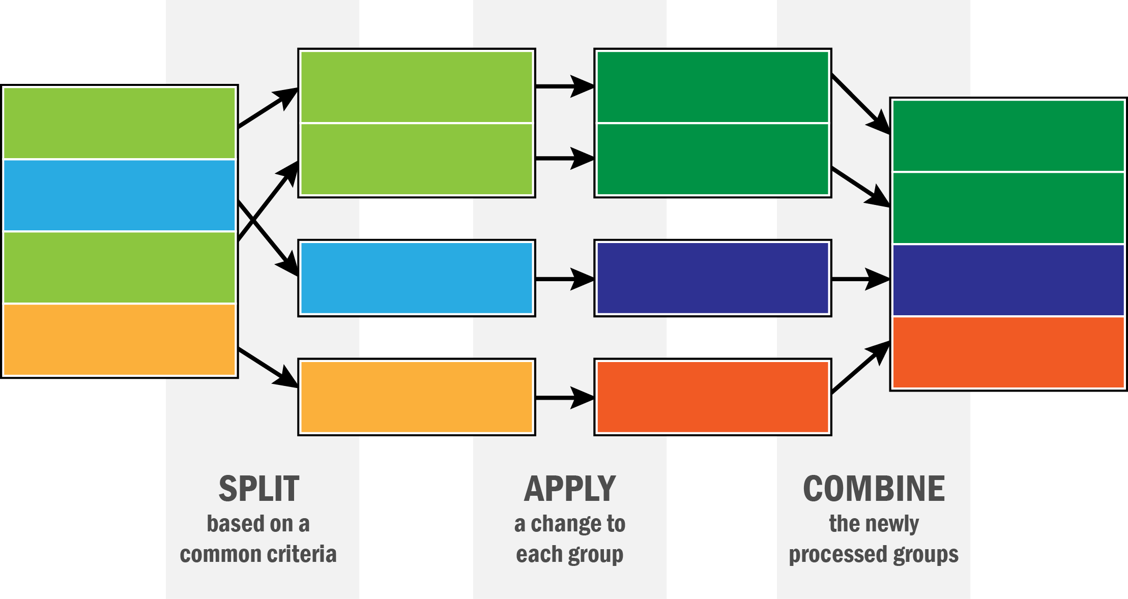
Data aggregation and split-apply-combine
gapminder =  pd.read_csv('data/gapminder.tsv', sep = '\t')
gapminder.head()
| country | continent | year | lifeExp | pop | gdpPercap | |
|---|---|---|---|---|---|---|
| 0 | Afghanistan | Asia | 1952 | 28.801 | 8425333 | 779.445314 |
| 1 | Afghanistan | Asia | 1957 | 30.332 | 9240934 | 820.853030 |
| 2 | Afghanistan | Asia | 1962 | 31.997 | 10267083 | 853.100710 |
| 3 | Afghanistan | Asia | 1967 | 34.020 | 11537966 | 836.197138 |
| 4 | Afghanistan | Asia | 1972 | 36.088 | 13079460 | 739.981106 |
gapminder.groupby('country')['lifeExp'].mean()
country
Afghanistan           37.478833
Albania               68.432917
Algeria               59.030167
Angola                37.883500
Argentina             69.060417
                        ...
Vietnam               57.479500
West Bank and Gaza    60.328667
Yemen, Rep.           46.780417
Zambia                45.996333
Zimbabwe              52.663167
Name: lifeExp, Length: 142, dtype: float64
gapminder.groupby('country').get_group('United Kingdom')
gapminder.groupby('continent').lifeExp.agg(np.median) # Medians
continent
Africa      47.7920
Americas    67.0480
Asia        61.7915
Europe      72.2410
Oceania     73.6650
Name: lifeExp, dtype: float64
gapminder.groupby('year').agg({'lifeExp': np.mean, 'pop': np.median, 'gdpPercap': np.median}).reset_index()
| year | lifeExp | pop | gdpPercap | |
|---|---|---|---|---|
| 0 | 1952 | 49.057620 | 3943953.0 | 1968.528344 |
| 1 | 1957 | 51.507401 | 4282942.0 | 2173.220291 |
| 2 | 1962 | 53.609249 | 4686039.5 | 2335.439533 |
| 3 | 1967 | 55.678290 | 5170175.5 | 2678.334741 |
| 4 | 1972 | 57.647386 | 5877996.5 | 3339.129407 |
| 5 | 1977 | 59.570157 | 6404036.5 | 3798.609244 |
| 6 | 1982 | 61.533197 | 7007320.0 | 4216.228428 |
| 7 | 1987 | 63.212613 | 7774861.5 | 4280.300366 |
| 8 | 1992 | 64.160338 | 8688686.5 | 4386.085502 |
| 9 | 1997 | 65.014676 | 9735063.5 | 4781.825478 |
| 10 | 2002 | 65.694923 | 10372918.5 | 5319.804524 |
| 11 | 2007 | 67.007423 | 10517531.0 | 6124.371109 |