Using Jupyter notebooks in the GLAM Workbench
The GLAM Workbench includes many Jupyter notebooks. Jupyter lets you combine text, images, and live code within a single web page. So not only can you read about collections data, you can download it, analyse it, and visualise it – all within your browser!
While notebooks often include some fairly intimidating looking code, you don't need to understand the code to use them. As explained below, there's just a couple of basic conventions you need to keep in mind when running Jupyter notebooks. Once you've mastered these, you'll be able to use any of the tools or examples in this workbench.
Of course, once you've developed a bit of confidence, you might want to start playing around with the code. That's how you learn. The GLAM Workbench isn't just a collection of tools, it's a starting point – from here you can explore, extend, and experiment!
1. Text cells and code cells
You're currently inside a Jupyter notebook. It might look like any old web page, but there are a number of important differences.
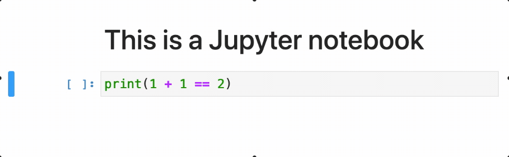
Jupyter notebooks contain two main components – text cells and code cells. This is a text cell. As well as ordinary text, these cells can contain things like links, images, and tables. Text cells are used to provide documentation and context.

Text cells can include images and links. All aboard the PS Jupiter, thanks to the State Library of South Australia!
Code cells are easy to identify, as they have boxes around them, like this:
# Hi there! I'm a code cell!

# Lines that begin with a hash symbol, like these, are comments within code.
# They don't do anything, but they help you understand how the code works.
Code cells contain snippets of live, executable code – they do things. It's this combination of documentation and real, live code examples that make Jupyter notebooks so useful. You can learn by doing!
2. Running a code cell
Most of the notebooks in the GLAM Workbench include snippets of real code. You can use this code to do things like download data, or create charts. The programming language used here is Python. It's popular in the data sciences and is generally pretty easy for humans to understand.
To run code cells:
- Click on the code cell (you'll see the cell becomes highlighted).
- Hit Shift+Enter (the code will run and you'll be moved on to the next cell).
- If the code cell generates an output, such as text or data, it'll be displayed below the cell.
That's it – try it with the cell below! If all goes well, you should see a message with today's date.
# CLICK ON ME AND THEN HIT SHIFT+ENTER!

# This makes the datetime module available to use
import datetime

# This creates a variable called 'date_now' and uses the datetime.date.today() function to set it to today's date.
date_now = datetime.date.today()

# This displays a nicely-formatted string containing the date
print(f'Congratulations! You ran the code in this cell on {date_now}.')
Help! Nothing happens when I click!
If nothing happens when you click on a cell or hit Shift+Enter it's probably because you're viewing a static version of the notebook. See Introduction for setting up a live version.
You can also run the code in a highlighted cell by clicking on the ▶ icon in the toolbar, or by hitting Control+Enter. You'll notice that Shift+Enter runs the code and moves you on to the next cell, while Control+Enter leaves you where you are.
3. Starting from the top
In the code cell above we created a variable called date_now. Variables are just labelled containers that we use to store values. In this case, date_now contains a representation of today's date.
Now that the date_now variable has been defined, we can use it in other places within this notebook. The cell below extracts the year component of date_now. Just click on the cell and hit Shift+Enter as before to view the result.
# Run me to see how we can access the 'date_now' variable

# This gets the year from the date stored in the date_now variable.
date_now.year
Help! I get a weird 'Name Error' saying that 'date_now is not defined.
If you get a message about a NameError, make sure that you've run the first code cell (where we create the 'date_now' variable, before this one. Most Jupyter notebooks expect you to run cells in order, from top to bottom.
Jupyter notebooks will often set up bits of code, like variables and functions, that are reused throughout the notebook. This means that usually best to run code cells in the order that they appear – working from the top to the bottom of the notebook. That way everything should be set up, ready to run as needed. If you get an error when you run a cell, check back to make sure all the relevant cells above it have been executed.
4. Status of a code cell
You might have noticed that after a code cell has been run a number appears in the square brackets – [ ]: to the left of the cell. This helps you keep track of which cells have been executed and when. While the code in a cell is running you'll see an asterisk – [*]:. This changes to a number once the code has completed.
In some cases, cells will start processes that take a bit of time to complete. For example, harvesting series data from RecordSearch can take lots of time depending on how big the series is. You won't be able to run any more cells until the current one has finished. Just wait for the asterisk to turn into a number and you'll be right to move on.
5. Editing a code cell
In many places throughout this workbench, you'll be asked to edit or add to the code. By doing that you can customise the code to your own research interests. Don't be intimidated – if something goes wrong, you can just try again. To edit a code cell:
- Click on the code cell to activate it.
- You'll see that the cursor turns into a normal text insertion cursor – just edit the code as you would any piece of text.
- When you've finished editing, make sure you hit Shift+Enter to run the cell. Your edits won't be visible to the notebook until the cell is run.

Try it in the cell below!
- Click on the cell to activate it.
- Select 'Tim' in the code and type in your own name. Make sure you keep the quotes around your name.
- When you've finished editing, hit Shift+Enter to run the cell.
The cell will save your name to the variable your_name, and then print a personalised greeting.
# Edit this cell to add your name between the quotes, and then run it
your_name = 'Tim' # <-- EDIT ME!

print(f'Hi {your_name}! Welcome to the OzGLAM workbench. 👋')
Help! I get a weird 'SyntaxError' or 'Name Error'.
Make sure your name is enclosed in quotes (either single or double, as long as they match). Quotes indicate that you're working with a string or text value. Without them, Python will go looking for a variable labelled with your name!
6. Let's try getting some data!
Once you know how to run and edit cells, you can start to do all sorts of interesting things – such as getting collection data from the National Museum of Australia!
The NMA makes its collection data available through an API (Application Programming Interface). This means we can fire off queries and get results back in a structured form that we can process and analyse. To do this, we'll make use of Requests – the go-to Python package for moving data around on the web.
There are three main steps in making an API request.
- Construct the request by setting API query parameters.
- Send the request off to the API.
- Do something with the data received from the API.
6.1. Construct the request
There are a large number of possible API query parameters you can use to search for objects in the NMA collection. To find objects matching a particular keyword, we can use the text parameter. We'll also use the limit parameter to tell the API we only want one record.
Here you can use you new code cell editing skills to set the keyword you want to search for. In the cell below:
- Click on the cell below to activate it.
- Look for the value 'stone' in the cell below and change it to something that you want to search for (but keep the quotation marks!).
- Run the cell using Shift+Enter.
# EDIT WHERE INDICATED THEN RUN THIS CELL!

your_keyword = 'stone'  # <-- EDIT ME! (But leave the quotes)

# Here we'll put our desired parameters into a variable called `params`
# In Python, this sort of variable is called a dictionary -- it contains a series of labelled values
params = {
    'text': your_keyword, # What we want to search for
    'limit': 1 # Give us 1 record only please!
}

# Display the contents of `params`
# This is what we'll send to the API
print(params)
Help! I get a weird 'SyntaxError' or 'Name Error'.
Make sure your keyword value is enclosed in quotes (either single or double, as long as they match).
6.2. Send the request to the API
Now we have our parameters, we need a url to send them to! The NMA API documentation lists a series of 'endpoints'. Each endpoint is a url that returns a particular type of data. To search for objects we need to send our requests to this url: https://data.nma.gov.au/object.
The cell below makes our request and saves the response to a variable called response. It then displays the status_code of our request – if everything went ok, the status_code should be '200'.
Run the cell below to send our request to the NMA API.
# RUN THIS CELL!

# This is how we import an external package or library into Python
# This loads the requests package so we can use it
import requests

# This is the base url we use to send our search terms to the NMA API.
url = 'https://data.nma.gov.au/object'

# Send our parameters to the object endpoint, saving the response in a variable
response = requests.get(url, params=params)

# Display the status code of our request
print(response.status_code)
6.3. Do something with the data
Now we can extract the API data from the response variable and display it.
Run the cell below to display the search data.
# RUN THIS CELL!

# We extract the results as JSON
results = response.json()

# Display the results
results
If your keyword can't be found, you'll see something like data: [] – indicating that the list of results is empty. Try changing the value of your_keyword in the cell under 6.1, then run the cells in 6.1 and 6.2 again to send the new request to the API. Keep trying until you get some data!
The data arrives back in a standard format known as JSON (JavaScript Object Notation). The main things to notice are that it contains labels and values, and these labels and values are arranged in some sort of hierarchy. If we understand the hierarchy, we can get back the value for any label – it's just a matter of following the path through the hierarchy until we get to the value we want. For example, here's how we get the value for title.
# RUN THIS CELL to get the value of `title`
results['data'][0]['title']
The [0] says that we want the first record contained within the result data (although in this case there's only one anyway).
You might also notice that meta includes a results value that tells us the total number of results matching our keyword. Here's how we get the to the results value.
# RUN THIS CELL to get the number of search results
results['meta']['results']
7. Let's make a dataset!
We made one request to the API and found out the number of items matching our keyword. By repeating this process multiple times with different keywords, we can start building up a picture of the NMA's holdings.
This time, instead of defining a single keyword, we'll create a list of keywords. Then we'll loop through the list of keywords, sending off API requests to get the total number of results for each. Once we have all the data, we'll use Pandas, the all-purpose (and frighteningly powerful) data analysis package, to convert our data into a dataframe. Dataframes come with with all sorts of useful built-in tools for shaping and analysing data.
7.1. Create a list of keywords
First let's create our list of keywords. Note than Python uses square brackets to define a list of values:
- Look for the line
keywords = ['cat', 'dog', 'kangaroo', 'koala']in the cell below – this creates a list of keyword values. - Edit the list – feel free to add, remove, or edit any of the keywords, but keep the quotes around each value, and the square brackets. You can include as many keywords as you want.
- Run the cell to save the list.
# EDIT AND RUN THIS CELL

# The square brackets indicate that this is a list of values
# Change or add values as you wish, but keep the square brackets!
keywords = ['cat', 'dog', 'kangaroo', 'koala'] # <-- EDIT ME TO ADD OR REMOVE KEYWORDS
7.2. Loop through the keyords getting the number of results for each
Now we're going to use the list of keywords to build a loop. A loop in Python repeats a set of instructions. In this case each iteration of the loop will search for one of the keywords, saving the total number of results.
Once the loop has finished, we'll have a new list called totals containing all the results we harvested.
Run the cell below to start the harvest. Because it makes multiple requests to the NMA API it will take a little while to complete. Remember to keep an eye on the square brackets to the left of the cell – when the asterisk becomes a number, it's finished!
# RUN THIS CELL

# We'll import time to insert a brief pause in our loop
import time

# This is an empty list to put our data in.
totals = []

# Create our params dictionary.
# We'll add the 'text' parameter inside the loop
params = {
    'limit': 1
}

# This is the base url we use to send our search terms to the NMA API.
url = 'https://data.nma.gov.au/object'

# We're going to loop through the keywords one at a time
for keyword in keywords:

    # We're inside the loop now!

    # Add the 'text' value to our parameters
    params['text'] = keyword

    # This is the same code we used above
    # Now it's in a loop, so it gets repeated multiple times

    # Make the API request
    response = requests.get(url, params=params)

    # Extract the JSON data
    data = response.json()

    # Get the total number of results
    total = data['meta']['results']

    # Now we'll save the keyword and the total results to our list
    totals.append({'keyword': keyword, 'total': total})

    # Anonymous access to the NMA API has usage limits -- here we put in a pause of 1 second to stay within the limits.
    time.sleep(1)

# Display the harvested data
totals
7.3. Convert the data to a Pandas dataframe
Pandas dataframes are very useful for exploring tabular data. They come with a lot of built-in tools that make it quick to analyse, manipulate, and summarise data. In the cell below we'll convert totals into a dataframe and display the result. Pandas is nicely integrated with Jupyter, so the dataframe will be automatically formatted as a table.
# RUN THIS CELL

# By convention pandas is assigned the shorthand 'pd' when we import it
import pandas as pd

# Now we'll convert our raw data into a Pandas dataframe
# Dataframes come with all sorts of useful methods for analysing/shaping data
df = pd.DataFrame(totals)

# Display the dataset
df
Our dataset is tiny, so it's easy to see what's going on. If you have lots of data, Pandas can help you make sense of it. For example, we might want to find the keyword with the highest number of results.
# RUN THIS CELL to find which row has the largest value
df.loc[df['total'].idxmax()]
Or perhaps you'd like to know the total number of search results across all keywords.
# RUN THIS CELL to get the sum of all values
df['total'].sum()
These are just a couple of examples of how Pandas helps you work with tabular data. There are many more throughout the GLAM workbench!
8. Let's try visualising our dataset
We've displayed our data as a table, but a chart would be easier to interpret at a glance. There are a number of charting and data visualisation packages available for Python, here we'll be using Altair. You just feed Altair a dataframe, and tell it the columns to display on each axis. Let's start with a simple bar chart that shows the keywords along the x axis, and the number of search results on the y axis.
import altair as alt

# Create a new chart using our dataframe
alt.Chart(df).mark_bar().encode(
    x='keyword:N', # Show the keyword on the X axis
    y='total:Q', # Show the number of results on the Y axis
    tooltip=['keyword', 'total'] # Tooltips display when you mouseover the chart
)
Altair is easy to customise. Here's a few things you could try:
- Switch the
xandyvalues in the code above and see what happens. - Change
mark_bartomark_line.
9. Save our dataset as a CSV file
Many of the notebooks in the GLAM Workbench help you harvest data from GLAM collections, just as we did above. Once you've created a new dataset, you'll probably want to save it. Pandas makes it easy to save your dataframe as a CSV (Comma Separated Values) file. CSV files are simple text files that can be opened by any spreadsheet program. They're widely used for storing and sharing datasets.
# RUN THIS CELL to save your dataset as a CSV file

# This is the filename we'll use for the CSV file, edit if you want
csv_file = 'my_nma_dataset.csv'  # <-- EDIT ME if you'd prefer a different filename

# Save the dataframe as a CSV file
df.to_csv(csv_file, index=False)
Once you've created your CSV file you can download it from Jupyter to your local computer. The cell below will create a handy link to the file.
# RUN THIS CELL to create a link to the CSV file
from IPython.display import display, HTML

# Display a link to the CSV file
display(HTML(f'<a href="{csv_file}" download>Download CSV file</a>'))
10. Next steps
This notebook has introduced you to the basics of Jupyter. You've learnt how to run and edit cells, but you've also harvested some data from an API, created a dataset, visualised the dataset, and saved it as a CSV file. As you work through the GLAM Workbench you'll find yourself repeating this sort of pattern – getting, analysing, and saving data. You've also met some important tools like Requests, Pandas, and Altair. Once again you'll find them popping up all over the place. The examples used in this notebook might have been pretty simple, but they provide a good introduction to what the GLAM Workbench is all about.
You also learnt a little bit of Python – variables, imports, lists, dictionaries, and loops. The GLAM Workbench isn't a 'learn to code' site, but as you work your way through the notebooks, you'll start to recognise some familiar patterns in the code as well. If you'd like to learn more about Python, work your way through this excellent set of notebooks by Nathan Kelber and Ted Lawless:
Created by Tim Sherratt (@wragge) for the GLAM workbench. If you think this project is worthwhile you can become a GitHub Sponsor.