Notebook

Subsurface Data Analytics¶

Introduction to Artificial Neural Networks: Single Layer ANN¶

John Eric McCarthy II, Undergraduate Student, The University of Texas at Austin¶

LinkedIn ¶

Supervised by:¶

Michael Pyrcz, Professor, The University of Texas at Austin¶

Twitter | GitHub | Website | GoogleScholar | Book | YouTube | LinkedIn | GeostatsPy ¶

Neural Networks¶

Artificial neural networks or ANNs are modeled after a human's neural network in the sense that they receive inputs, interpret those inputs, and output the result of that interpretation. There are many different variants of ANNs. For this workflow, we will be examining the different aspects of a single layer neural network:

Input layer
Hidden layer
Output layer
Weights
Learning Rate

Real Life Application¶

Today, ANNs are used to solve problems and make predictions by finding complex relationships between inputs and outputs. Forecasting, customer research, data validation, and risk management are some of the many problems that businesses use ANNs to solve. Oil and gas companies have been optimizing their operations with machine learning for many years. Machine learning has been commonly used for enhanced reservoir modeling, allowing users to predict how formations will react to certain drilling techniques.

Workflow Goals¶

Learn the basics of machine learning in python to predict subsurface features. This includes:

Loading and visualizing sample data
Developing a basic understanding of neural networks

Getting Started¶

The following data files are available for you to download into your working directory. That raw data data files and images are already built into the workflow, but they are available here:

Tabular data - Stochastic_1D_por_perm_demo.csv
Tabular data - Random_Parabola.csv

These datasets are available in the folder: https://github.com/GeostatsGuy/GeoDataSets.

And the following images:

The images are available in the folder: https://github.com/GeostatsGuy/Resources.

Import Required Packages¶

We will also need some standard packages. These should have been installed with Anaconda 3.

In [1]:

import numpy as np                                                     # ndarrys for gridded data
import pandas as pd                                                    # DataFrames for tabular data
import os                                                              # set working directory, run executables
import matplotlib.pyplot as plt                                        # for plotting
import matplotlib.image as mpimg 
import seaborn as sns                                                  # for plotting
import warnings                                                        # supress warnings from seaborn pairplot
from sklearn.model_selection import train_test_split                   # train / test DatFrame split
from sklearn.pipeline import Pipeline                                  # for polynomial regression
from sklearn.preprocessing import PolynomialFeatures
from sklearn.linear_model import LinearRegression
from sklearn.model_selection import cross_val_score
from IPython.core.display import display, Javascript, clear_output
from IPython.display import Markdown as md
%matplotlib inline                        

The following workflow has been made interactive through the use of ipywidgets.

Instructions for installation of this package can be found here

In [2]:

from ipywidgets import *                                               # import shortcut for widgets

We will also need the following packages to train and test our artificial neural nets:

Tensorflow - open source machine learning
Keras - high level application programing interface (API) to build and train models

More information is available at tensorflow install.

You can find great instructions for installation with Anaconda here!

This workflow was designed with tensorflow version 2.1.0

To check your current version of tensorflow you could run the next block of code.

In [3]:

import tensorflow as tf
from tensorflow.keras.models import Sequential, load_model
from tensorflow.keras.layers import Dense, Dropout, Activation
import tensorflow.keras as keras
from tensorflow.python.keras import backend as k
tf.__version__                                                         # check the installed version of tensorflow

Out[3]:

'2.1.0'

Set the working directory¶

I always like to do this so I don't lose files and to simplify subsequent read and writes (avoid including the full address each time).

by running the following code you will be able to see the current directory that you are working in

os.getcwd()

make sure that all of the files listed above are saved there. Otherwise, specify the file location with:

os.chdir()

In [4]:

os.getcwd()                                                            # get the current working directory

Out[4]:

'C:\\Users\\jmcca\\PGE383'

We will now set the working directory. In the cell below, replace os.getcwd() with the file path if you do not wish to save the images and the .csv files in the same folder as this workflow.

In [5]:

os.chdir(os.getcwd())                                                  # set the working directory

Loading Data¶

Let's load the provided multivariate, spatial dataset 'Stochastic_1D_por_perm_demo.csv'. It is a comma delimited file with:

Porosity
Permeability

It is common to transform properties to a standard normal for geostatistical workflows.

We load it with the pandas 'read_csv' function into a data frame we called 'df' and then preview it to make sure it loaded correctly.

Python Tip: using functions from a package just type the label for the package that we declared at the beginning:

import pandas as pd

so we can access the pandas function 'read_csv' with the command:

pd.read_csv()

but read csv has required input parameters. The essential one is the name of the file. For our circumstance all the other default parameters are fine. If you want to see all the possible parameters for this function, just go to the docs here.

The docs are always helpful
There is often a lot of flexibility for Python functions, possible through using various inputs parameters

also, the program has an output, a pandas DataFrame loaded from the data. So we have to specficy the name / variable representing that new object.

df = pd.read_csv('Stochastic_1D_por_perm_demo.csv')

Let's run this command to load the data and then look at the resulting DataFrame to ensure that we loaded it.

In [6]:

df = pd.read_csv(r'https://raw.githubusercontent.com/GeostatsGuy/GeoDataSets/master/Stochastic_1D_por_perm_demo.csv')         # read a .csv file in as a DataFrame
df.head()                                                   # we could also use this command for a table preview 

Out[6]:

	Unnamed: 0	Porosity	Permeability
0	0	13.746408	193.721529
1	1	9.608479	105.718666
2	2	11.664361	138.539297
3	3	8.375338	93.719985
4	4	13.183358	169.738825

In [7]:

for x in df.columns:                                        # find the names of the columns!
    print(x)                                                # other option is:      list(df.columns)        

Unnamed: 0
Porosity
Permeability

In [8]:

df = df.drop("Unnamed: 0", axis=1)                          #drop the unnecessary column
df.head()

Out[8]:

	Porosity	Permeability
0	13.746408	193.721529
1	9.608479	105.718666
2	11.664361	138.539297
3	8.375338	93.719985
4	13.183358	169.738825

Data Normalization¶

We must normalize the features before we apply them in an artificial neural network model. These are the motivations for this normalization:

remove the impact of scale when using different types of data
activation functions in artificial neural networks are designed to be more sensitive to values of nodes closer to 0.0 (i.e., results in higher gradient and improves backpropagation in training)

Lets get the minimums and maximums of our data first:

In [9]:

# find the minimums and maximums of the data

por_min = df['Porosity'].values.min()
print("The minimum value in the Porosity column is: " + str(por_min))
por_max = df['Porosity'].values.max()
print("The maximum value in the Porosity column is: " + str(por_max))
perm_min = df['Permeability'].values.min()
print("The minimum value in the Permeability column is: " + str(perm_min))
perm_max = df['Permeability'].values.max()
print("The maximum value in the Permeability column is: " + str(perm_max))

The minimum value in the Porosity column is: 3.2587377609366293
The maximum value in the Porosity column is: 21.68483990762835
The minimum value in the Permeability column is: 44.50587461913492
The maximum value in the Permeability column is: 605.7101403233376

Normalization Formula¶

\begin{equation} X_{normalized} =\frac{X - X_{minimum}}{X_{maximum}-X_{minimum}} \end{equation}

Let's normalize each feature.

We apply the min max normalization by-hand to force both the predictor and response features to be bound $[-1,1]$.
It is easy to backtransform given we keep track of the original min and max values

In [10]:

df['norm_Porosity'] = (df['Porosity'] - por_min)/(por_max - por_min) * 2 - 1          # normalize porosity to range from 0 to 1
df['norm_Permeability'] = (df['Permeability'] - perm_min)/(perm_max - perm_min) * 2 - 1         # normalize permeability to range from -1 to 1
df['n_Perm_zero_to_one'] = (df['Permeability'] - perm_min)/(perm_max - perm_min)      # normalize permeability to range from 0 to 1

df.head()

Out[10]:

	Porosity	Permeability	norm_Porosity	norm_Permeability	n_Perm_zero_to_one
0	13.746408	193.721529	0.138349	-0.468231	0.265885
1	9.608479	105.718666	-0.310788	-0.781852	0.109074
2	11.664361	138.539297	-0.087640	-0.664887	0.167557
3	8.375338	93.719985	-0.444636	-0.824612	0.087694
4	13.183358	169.738825	0.077235	-0.553699	0.223150

It is also a good idea to check the summary statistics.

All normalized features should now range from -1 to 1 or 0 to 1

In [11]:

df.describe().transpose()

Out[11]:

	count	mean	std	min	25%	50%	75%	max
Porosity	105.0	11.996402	3.620428	3.258738	9.572742	11.664361	14.209854	21.68484
Permeability	105.0	170.010310	95.378037	44.505875	104.656351	139.628789	200.101407	605.71014
norm_Porosity	105.0	-0.051599	0.392967	-1.000000	-0.314667	-0.087640	0.188653	1.00000
norm_Permeability	105.0	-0.552732	0.339905	-1.000000	-0.785638	-0.661004	-0.445494	1.00000
n_Perm_zero_to_one	105.0	0.223634	0.169952	0.000000	0.107181	0.169498	0.277253	1.00000

Activation Functions¶

The purpose of an activation function is to add a non-linear property to the function. Every node in a neural network has two jobs:

Linear Summation
Activation Computation

The activation function continuously fires while the ANN is in use. This is done by calculating the weighted sum of the inputs, adding a bias, and introducing non-linearity to the ouput. Without the activation function, our model will not be able to learn and will be limited in complexity.

Sigmoid Function¶

A sigmoid function has an "S" shaped curve that ranges from 0 to 1. This function is commonly used in models that need to predict probability as an output.

\begin{equation}¶

f(x) = \frac{1}{1 + e^{-x}} \end{equation}

Tanh Function¶

The hyperbolic tangent (tanh) function is similar to the sigmoid function. The advantage in using tanh is that it ranges from -1 to 1. This means that strong negative and postive outputs will be mapped as such while inputs with a value of zero will remain near zero.

\begin{equation}¶

f(x) = \frac{e^{x} - {e^{-x}}}{e^{x} + e^{-x}} \end{equation}

ReLU Function¶

The rectified linear units function (ReLU) is the most popular activation function. This function ranges from 0 to infinity. If the input is positive, the ouput is the same as the input. Otherwise, the output is 0.

\begin{equation}¶

f(x) = max(0, x) \end{equation}

Below we will create plots for each function and widget sliders that control the inputs.

In [12]:

# create title

l = widgets.Text(value='                                Artificial Neural Networks Activation Function Demo, John Eric McCarthy II and Michael Pyrcz, The University of Texas at Austin',
                 layout=Layout(width='950px', height='30px'))

# create slider for each activation function

xs = widgets.FloatSlider(min=-10.0, max = 10.0, step = .1, value=0, description = 'X',orientation='horizontal', continuous_update=True)
xs.style.handle_color = 'red'
xt = widgets.FloatSlider(min=-10.0, max = 10.0, value=0, description = 'X',orientation='horizontal', continuous_update=True)
xt.style.handle_color = 'yellow'
xr = widgets.FloatSlider(min=-1.0, max = 1.0, value=0, description = 'X',orientation='horizontal', continuous_update=True)
xr.style.handle_color = 'orange'

# create activation function plots

def sigmoid(xs):

    y = 1/(1 + np.exp(-xs))                                                                        # function for dot connected to slider
    plt.figure(figsize=(7.5,5))
    plt.title('Sigmoid Function', fontsize=20)  
    plt.xlabel("Input") 
    plt.ylabel("Output") 
    plt.ylim(-1.1,1.1)
    plt.xlim(-10,10)
    x1 = np.linspace(-10, 10, 100)
    y1 = 1/(1 + np.exp(-x1))                                                                      # function for line plot
    plt.plot(x1,y1,'-',color='black')
    plt.plot(xs,y,'o', markerfacecolor='red', markeredgecolor='black', markersize=20, alpha=1)
    plt.grid(True)
    plt.show()
    print('\033[1m' + 'f({}) =  {}'.format(xs, 1/(1 + np.exp(-xs))))
        
def tanh(xt):
    y = np.tanh(xt)                                                                               # function for dot connected to slider
    plt.figure(figsize=(7.5,5))
    plt.title('Tanh Function', fontsize=20)  
    plt.xlabel("Input") 
    plt.ylabel("Output") 
    plt.ylim(-1.1,1.1)
    plt.xlim(-10,10)
    x1 = np.linspace(-10, 10, 100)
    y1 = np.tanh(x1)                                                                              # function for line plot
    plt.plot(x1,y1,'-',color='black')
    plt.plot(xt,y,'o', markerfacecolor='yellow', markeredgecolor='black', markersize=20, alpha=1)
    plt.grid(True)
    plt.show()
    print('\033[1m' + 'f({}) =  {}'.format(xt, np.tanh(xt)))
        
def relu(xr):
    if xr < 0:                                                                                    # function for dot connected to slider
        y = 0
    if xr >= 0:
        y = xr
    plt.figure(figsize=(7.5,5))
    plt.title('ReLU Function', fontsize=20)  
    plt.xlabel("Input") 
    plt.ylabel("Output") 
    plt.ylim(-1,1)
    plt.xlim(-1,1)
    x1 = np.linspace(-1.1, 1.1, 1000)
    zero = np.zeros(len(x1))
    y1 = np.max([zero, x1], axis=0)                                                               # function for line plot
    plt.plot(x1,y1,'-',color='black')
    plt.plot(xr,y,'o', markerfacecolor='orange', markeredgecolor='black', markersize=20, alpha=1)
    plt.grid(True)
    plt.show()
    if xr < 0:
        print('\033[1m' + 'f({}) =  {}'.format(xr, 0))
    if xr >= 0:
        print('\033[1m' + 'f({}) =  {}'.format(xr, xr))
        
        
interactive_plot1 = widgets.interactive_output(sigmoid, {'xs': xs})
interactive_plot1.clear_output(wait = True)                                                       # reduce flickering by delaying plot updating

interactive_plot2 = widgets.interactive_output(tanh, {'xt': xt})
interactive_plot2.clear_output(wait = True)                                                       # reduce flickering by delaying plot updating

interactive_plot3 = widgets.interactive_output(relu, {'xr': xr})
interactive_plot3.clear_output(wait = True)                                                       # reduce flickering by delaying plot updating

# create dashboard/formatting

uia = widgets.HBox([interactive_plot1],)
uia2 = widgets.VBox([xs, uia],)

uib = widgets.HBox([interactive_plot2],)
uib2 = widgets.VBox([xt, uib],)

uic = widgets.HBox([interactive_plot3],)
uic2 = widgets.VBox([xr, uic],)

uid = widgets.HBox([uia2,uib2,uic2],)
uid2 = widgets.VBox([l, uid],)

Interactive Activation Function Demonstration¶

select the inputs and observe the outputs of the activation functions
interactive plot demonstration with ipywidgets, matplotlib packages

John Eric McCarthy II, Undergraduate Student, The University of Texas at Austin¶

LinkedIn ¶

Michael Pyrcz, Associate Professor, University of Texas at Austin¶

Twitter | GitHub | Website | GoogleScholar | Book | YouTube | LinkedIn | GeostatsPy ¶

The Inputs¶

Select the inputs for each function:

X is the input computed by the activation function
f(x) is the output of the activation function

In [13]:

display(uid2)                            # display the interactive plots

VBox(children=(Text(value='                                Artificial Neural Networks Activation Function Demo…

Interactive Neural Network¶

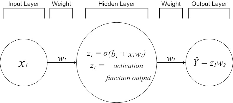
Neural networks have 3 main layers known as the input, hidden, and output layers. Each layer is responsible for executing a task and holds a collection of nodes. A single node in a layer is connected to every node in the next layer. Each connection has a weight applied to it. The output of a node is multiplied by a weight before it is passed on as an input. The input layer contains the predictor features and is the very beginning of the workflow. The hidden layers are any layers between the input and output layers. Deep Learning is the use of more than one hidden layer. You will be able to experiment with this at end of this workflow. Nodes located in the hidden layers take in a weighted sum of the outputs from the previous layer and produce an output through an activation function. The output layer is the last layer of nodes. This layer contains the output(s) of the hidden layer(s) and does not interact with the rest of the ANN.

Putting it all together¶

Below you will be tasked with becoming a neural network. Try your best to fit the data by adjusting the weights and bias of the ANN.

Notice:

The importance of normalizing the dataset beforehand
Through trial and error, it becomes easier to fit the data
The weights and bias that work with one activation function won't work with another
Some activation functions work better than others with this dataset

Below we will create the the widgets and plots that change depending on the activation function and inputs.

In [14]:

# create title

l = widgets.Text(value='                                    Simple Artificial Neural Network Demo, John Eric McCarthy II and Michael Pyrcz, The University of Texas at Austin',
                 layout=Layout(width='950px', height='30px'))

# create dropdown menu

act_func = widgets.Dropdown(options=['Sigmoid', 'Tanh', 'ReLU'], value='ReLU', description='Act. Funtion:', disabled=False, layout=Layout(width='200px', height='30px'), style = {'description_width': 'initial'})

# sliders for hyperparameters

w1 = widgets.FloatSlider(min=-5.00, max = 5.00, value=1.20, description = 'Weight 1',orientation='horizontal', continuous_update=False)
w1.style.handle_color = 'blue'
b1 = widgets.FloatSlider(min=-5.00, max = 5.00, value=1.20, description = 'Bias 1',orientation='horizontal', continuous_update=False)
b1.style.handle_color = 'red'
w2 = widgets.FloatSlider(min=-5.00, max = 5.00, value=0.41, description = 'Weight 2',orientation='horizontal', continuous_update=False)
w2.style.handle_color = 'green'


def update_plot(w1, w2, b1, act_func):                    # create plots
    
    x = np.linspace(-2, 2, 1000)    
    x1 = (x * w1) + b1
    if act_func == 'Sigmoid':
        y = 1/(1 + np.exp(-x1))                           # sigmoid function

    elif act_func == 'Tanh':
            y = np.tanh(x1)                               # tanh function

    elif act_func == 'ReLU':
        zero = np.zeros(len(x1))
        y = np.max([zero, x1], axis=0)                    # relu function
    
    x2 = (y * w2)
    
    if act_func == 'Sigmoid':
        y2 = 1/(1 + np.exp(-x2)) 

    elif act_func == 'Tanh':
        y2 = np.tanh(x2)

    elif act_func == 'ReLU':
        zero = np.zeros(len(x2))
        y2 = np.max([zero, x2], axis=0)
    fig = plt.subplots(figsize=(15, 5))
    plt.title('Interactive Neural Network: "Inter- net"', fontsize=20)
    plt.plot(x, y2)
    if act_func == 'Sigmoid' or 'ReLU':
        y_values = df['n_Perm_zero_to_one'].values
    if act_func == 'Tanh':
        y_values = df['norm_Permeability'].values
    
    plt.plot(df['norm_Porosity'].values,y_values, 'o', markerfacecolor='red', markeredgecolor='black', alpha=0.7, label = "Test Data")
    if act_func == 'Sigmoid' or 'ReLU':
        y_min = -.1
    if act_func == 'Tanh':
        y_min = -1.1
    plt.ylim(y_min,1.1)
    plt.xlim(-1.1,1.1)
    plt.xlabel("Porosity") 
    plt.ylabel("Permeability") 
    plt.legend()
    plt.show()

def ann_plot(w1, b1, w2):                                 # display input and output of function
    
    img = mpimg.imread(r"https://raw.githubusercontent.com/GeostatsGuy/Resources/master/EmptyNeuralNet1.png")
    plt.figure(figsize=(15,12.5))
    plt.text(350,190, b1,{'color': 'red', 'fontsize': 24})
    plt.text(465,190, w1,{'color': 'blue', 'fontsize': 24})
    plt.text(190,200, w1,{'color': 'blue', 'fontsize': 24})
    plt.text(735,225, w2,{'color': 'green', 'fontsize': 24})
    plt.text(555,200, w2,{'color': 'green', 'fontsize': 24})
    plot = plt.imshow(img) 
    plt.axis('off')                                       # clear x-axis and y-axis
    
interactive_plot = widgets.interactive_output(update_plot, {'act_func': act_func,'w1': w1, 'b1': b1, 'w2': w2})
interactive_plot.clear_output(wait = True)                # reduce flickering by delaying plot updating

update_ann = widgets.interactive_output(ann_plot, {'w1': w1, 'b1': b1, 'w2': w2})

# create dashboard/formatting

ui = widgets.HBox([act_func],)                            # basic widget formatting 
uia = widgets.HBox([w1,b1,w2],)
uib = widgets.HBox([ui, uia])
uic = widgets.HBox([interactive_plot, update_ann])

Interactive Neural Network Demonstration¶

adjust the hyperparameter and select the activation function
observe the fit across the test data
interactive plot demonstration with ipywidgets, matplotlib packages

John Eric McCarthy II, Undergraduate Student, The University of Texas at Austin¶

LinkedIn ¶

Michael Pyrcz, Associate Professor, University of Texas at Austin¶

Twitter | GitHub | Website | GoogleScholar | Book | YouTube | LinkedIn | GeostatsPy ¶

The Inputs¶

Interact with the widgets to adjust the hyperparameters and fit the data provided

weight 1 is multiplied times each input before it is passed to the hidden layer
bias 1 is added to the product of the input and weight 1
weight 2 is multiplied times the output of the hidden layer once the activation function computation is done

In [15]:

display(l, uib, uic)                                              # display the interactive plot

Text(value='                                    Simple Artificial Neural Network Demo, John Eric McCarthy II a…

HBox(children=(HBox(children=(Dropdown(description='Act. Funtion:', index=2, layout=Layout(height='30px', widt…

HBox(children=(Output(), Output()))

Single Layer Neural Network¶

Increased Complexity¶

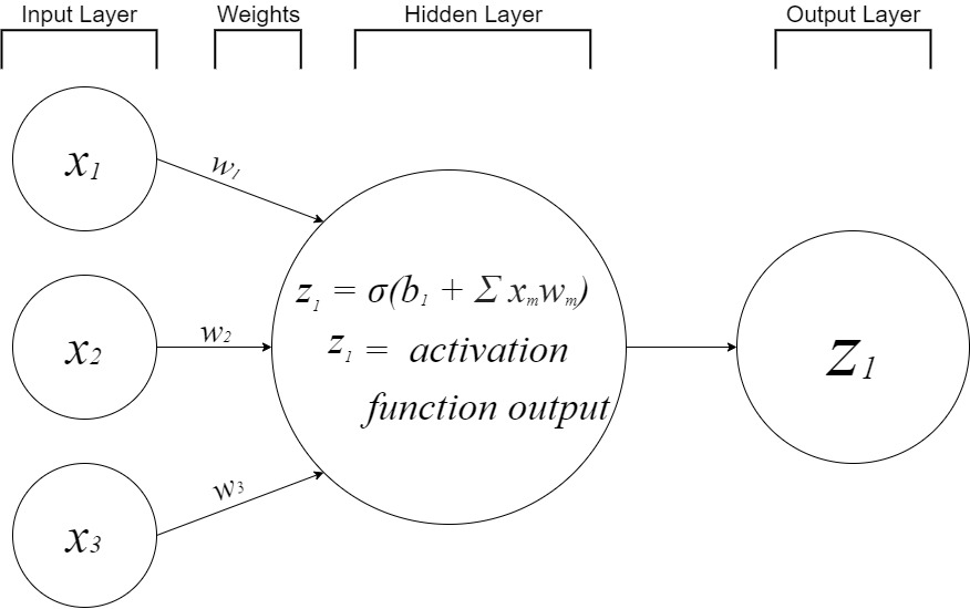
Below, you can find a new neural network that receives 3 inputs and predicts the output. Since we are predicting probability, we will be using the sigmoid activation function. The hidden layer creates a weighted sum of the inputs and adds a bias. This is equivalent to "s". Next, the activation function takes "s" as an input and the result is sent to the output layer. By design choice and for the sake of simplicity, there will not be a weight between the hidden and output layer for this example. This is great, but how does our ANN learn?

Introducing Backpropagation¶

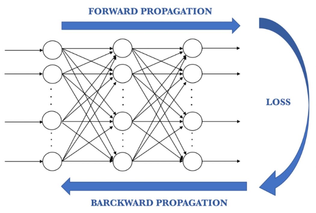
The process of running inputs through the neural network and receiving an output is called forward propagation or feed forward. ANNs require training and adjustment in order to learn. The weights between each node are the only thing that we have control over when it comes to changing our outputs. Below, we use batch gradient descent to adjust our weights throughout training. This is done by comparing the predicted result to the actual result and measuring the generated error. The learning rate affects how fast our neural network learns, or in other words, how much the weights are updated. We then back-propagate our error and repeat the process by passing our training data through the ANN. Back propagation is an algorithm for supervised learning that forces the ANN to "learn from mistakes". There are two main ways that an ANN can learn. In a supervised learning model, the ANN learns on a labeled dataset, providing an answer key that the ANN can use to evaluate its accuracy on training data. An unsupervised learning model, in contrast, provides unlabeled data that the ANN tries to make sense of by extracting features and patterns on its own.

When we update the weights we have to make a few simple calculations. First, we find the error by calculating the difference between the desired and actual output. We then multiply this by the learning rate to find the error rate. Next, we multiply the error rate by the input and the gradient (derivative) of the activation function. Design has gone into the creation of activation functions that make them relatively easy to calculate. In our ANN below, we use the sigmoid function because its derivative is actually just itself times 1 minus itself. Super cool! Although these calculations are simple, they do stack up fast.

Our goal is to minimize the error or cost. The cost can be calculated by finding the squared difference between the desired and actual output after each iteration. We will plot both the weight and cost changes of the ANN while it trains below.

How it Works¶

This neural network accepts 3 inputs: x1, x2, and x3. Based off of those inputs, a number is then predicted by the ANN. Below is a set of data that contains information on 4 animals. The ANN predicts the likelihood of an animal being a mammal or not based on: if it has hair, the number of legs it has, and the number of eyes it has. We will begin by extracting features from the dataset to put into our ANN. Then, we will classify the data by converting the data into 0s and 1s.

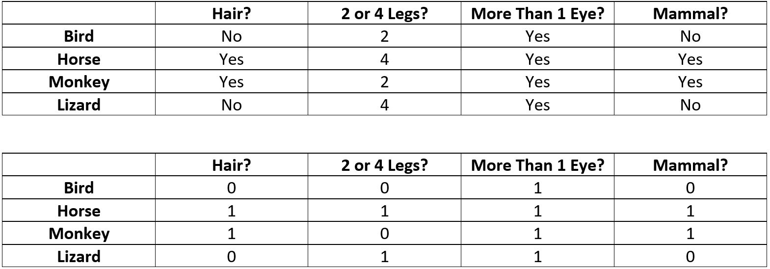
Input Layer:

Hair?
- No = 0
- Yes = 1
2 or 4 Legs?
- 2 Legs = 0
- 4 Legs = 1
More Than 1 Eye?
- More than 1 Eye = 1
- 1 Eye or Less = 0

Output Layer:

Mammal?
- No = 0
- Yes = 1

Below we will create an ANN that uses the above as a guide for the inputs and outputs. While training the model we will backpropagate the error and adjust the weights. We will also record the cost function throughout training.

In [16]:

# create title

l = widgets.Text(value='                                        Mammal Prediction Demo, John Eric McCarthy II, Undergraduate Student, The University of Texas at Austin',
                 layout=Layout(width='950px', height='30px'))

# create dropdown menus

hair = widgets.Dropdown(options=['Yes', 'No'], value='Yes', description='Hair?', disabled=False, layout=Layout(width='100px', height='30px'), style = {'description_width': 'initial'})
legs = widgets.Dropdown(options=['2', '4'], value='2', description='Number of Legs?', disabled=False, layout=Layout(width='150px', height='30px'), style = {'description_width': 'initial'})
n_eyes = widgets.Dropdown(options=['Yes', 'No'], value='Yes', description='More than 1 eye?', disabled=False, layout=Layout(width='175px', height='30px'), style = {'description_width': 'initial'})

class NeuralNetwork():
    
    def __init__(self):
        
        np.random.seed(1)                                                      # seed the random number generator 
        self.weights = 2 * np.random.random((3, 1)) - 1                        # set the weights to a 3x1 matrix with values from -1 to 1 and mean 0
        self.weight_change = np.empty((3,3,1))                                 # capture the weights after each iteration
        self.learning_rate = 1                                                 # define the learning rate of the model
        self.cost = np.empty((1,4,1))                                          # create an empty array to store the cost function values
        
    def sigmoid(self, x):                                                      # the sigmoid function takes in the weighted sum of the inputs and outputs a number between 0 and 1

        return 1 / (1 + np.exp(-x))

    def sigmoid_derivative(self, x):                                           # the derivative of the sigmoid function used to calculate necessary weight adjustments

        return x * (1 - x)

    def train(self, training_inputs, training_outputs, epochs):                # train the model by evaluating the error and adjusting the weights to get better results
        
        for iteration in range(epochs):                                        # pass training set through the neural network
            
            output = self.think(training_inputs)

            
            error = (training_outputs - output) * self.learning_rate           # calculate the error rate

                                                                               # multiply error by input and gradient of the sigmoid function
                                                                               # less confident weights are adjusted more through the nature of the function
            adjustments = np.dot(training_inputs.T, error * self.sigmoid_derivative(output))

            
            self.weights += adjustments                                        # adjust synaptic weights
            
                                                                               # store new weight values
            self.weight_change = np.append(self.weight_change, [self.weights], axis=0)
            
                                                                               # evaluate the cost function
            loss_error = 0
            loss_error += (training_outputs - output) ** 2
            self.cost = np.append(self.cost, [loss_error], axis=0)
            

    def think(self, inputs):                                                   # run the inputs through the neural network to get the outputs
        
        inputs = inputs.astype(float)
        output = self.sigmoid(np.dot(inputs, self.weights))
        return output

if __name__ == "__main__":                                                     # initialize the single neuron neural network
    
    neural_network = NeuralNetwork()

    print("Random starting weights: ")
    print(neural_network.weights)

    training_inputs = np.array([[0,0,1],                                      # the training set, with 4 examples consisting of 3 input values and 1 output value
                                [1,1,1],
                                [1,0,1],
                                [0,1,1]])

    training_outputs = np.array([[0,1,1,0]]).T                                # 4 output values

    neural_network.train(training_inputs, training_outputs, 10000)            # train the neural network

    print("Weights after training: ")
    print(neural_network.weights)

def test_ann(hair, legs, n_eyes):

    if hair == 'Yes':
        x1 = 1
    if hair == 'No':
            x1 = 0
    if legs == '2':
        x2 = 0
    if legs == '4':
            x2 = 2
    if n_eyes == 'Yes':
        x3 = 1
    if n_eyes == 'No':
            x3 = 0   

    probability = neural_network.think(np.array([x1, x2, x3]))
    if probability > .5:
        print('\033[1m' + 'The probability of the animal being a mammal is {}%'.format(np.round(probability * 100),2))
    if probability < .5:
        print('\033[1m' + 'The probability of the animal not being a mammal is {}%'.format(np.round(100 - (probability * 100),2)))
    if probability == .5:
        print('\033[1m' + 'The probability of the animal being a mammal is {}% \nThis is due to the nature of the sigmoid function. When all inputs are "0", .5 is returned by the function '.format(np.round(100 - (probability * 100),2)))


weight1 = neural_network.weight_change[:,0]                                    # store 3 weight changes for later use
weight2 = neural_network.weight_change[:,1]
weight3 = neural_network.weight_change[:,2]

cost2 = np.sum(neural_network.cost, axis = 1)                                  # store sum of costs

Random starting weights: 
[[-0.16595599]
 [ 0.44064899]
 [-0.99977125]]
Weights after training: 
[[ 9.67299303]
 [-0.2078435 ]
 [-4.62963669]]

In [17]:

# plot weight change and cost function

def weight_plot():
    fig = plt.subplots(figsize=(15, 5))
    plt.title('Weight Change Across Epochs', fontsize=20)
    x = np.linspace(0, len(neural_network.weight_change[:,0]), len(neural_network.weight_change[:,0]))    
    plt.plot(x, weight1, label = 'Weight 1')
    plt.plot(x,weight2, label = 'Weight 2')
    plt.plot(x,weight3, label = 'Weight 3')
    plt.ylim(-5,10)
    plt.xlim(0,len(neural_network.weight_change[:,0] + 100))
    plt.xlabel("Epochs") 
    plt.ylabel("Weight Change") 
    plt.legend()
    plt.show()

def cost_plot():   
    fig = plt.subplots(figsize=(15, 5))
    plt.title('Cost Change Across Epochs', fontsize=20)
    x = np.linspace(0, len(cost2), len(cost2))    
    plt.plot(x, cost2, label = 'cost')
    plt.ylim(-.07,1.25)
    plt.xlim(0, 200)
    plt.xlabel("Epochs") 
    plt.ylabel("cost") 
    plt.legend()
    plt.show()

show_probability = widgets.interactive_output(test_ann,{'hair': hair, 'legs': legs, 'n_eyes': n_eyes})
show_probability.clear_output(wait = True)                                     # reduce flickering by delaying plot updating   
weight_plot = widgets.interactive_output(weight_plot, {})
cost_plot = widgets.interactive_output(cost_plot, {})

# create dashboard/formatting

uia = widgets.HBox([hair, legs, n_eyes],)
uib = widgets.HBox([weight_plot, cost_plot],)

Interactive Predictive Neural Network Demonstration¶

test the neural network by answering the given questions
interactive plot demonstration with ipywidgets, matplotlib packages

John Eric McCarthy II, Undergraduate Student, The University of Texas at Austin¶

LinkedIn ¶

Michael Pyrcz, Associate Professor, University of Texas at Austin¶

Twitter | GitHub | Website | GoogleScholar | Book | YouTube | LinkedIn | GeostatsPy ¶

The Inputs¶

Answer the following questions to find out the probability of an animal with those features being a mammal, based off of what the ANN learned:

Hair?
2 or 4 Legs?
More Than 1 Eye?

In [18]:

display(l, uia, show_probability, uib)                                                # display the interactive plot

Text(value='                                        Mammal Prediction Demo, John Eric McCarthy II, Undergradua…

HBox(children=(Dropdown(description='Hair?', layout=Layout(height='30px', width='100px'), options=('Yes', 'No'…

Output()

HBox(children=(Output(), Output()))

Overfitting and Underfitting¶

Advanced neural networks undergo a multitude of transformations and changes in the hopes that the model will be able to make accurate predictions regardless of the dataset it is provided. Part of that training may be the introduction of a validation dataset. The validation data is a set of sample of data used to provide an unbiased evaluation of a model fit on the training dataset while tuning model hyperparameters. When used, we are essentially asking the model, "Can you make accurate predictions when given a set of unknown inputs"? For successful models, the answer to that question is yes. The great thing about using a validation data set is that you know the expected outputs. This makes calculating error and seeing what went wrong, that much easier.

It's important to understand the general concept behind underfitting and overfitting, so let's run through a few real life examples. Overfitting is like using a very specific training set to learn. For example, if someone only used Shakspearean language to learn the English. That person would defnitely know English, however it would be a very specific version of it. This would lead to complications when trying to understand other English text. Underfitting is like trying to learn English by listening to episodes of Friends, but only listening to sentences that begin with "The", "I", and "A". The problem here is that these sentences are limited and are a poor representation of the language.

You can gain a general understanding of how the model performs by the comparing the bias of the training set and the variance of the validation set with the fit of the model. A high bias and variance leads to underfitting while a low bias and variance leads to overfitting. Below, you can find a visual representation of underfitting versus overfitting while observing statistical data.

Adding Gaussianly Distributed Noise to the Data¶

Here, we are going to add gaussianly distributed noise to the porosity and permeability data. Gaussianly distributed meaning that the numbers have a mean of 0. Noise meaning that the numbers around the mean are random.

Gaussian Distribution¶

In the demo below you will have control over $\sigma$, the standard deviation being added to the inputs and outputs. The standard deviation is the amount of variation or dispersion of our values. We will also be calculating the sample variance, sample standard deviation, and mean squared error.

\begin{equation}¶

y = \frac{1}{\sigma\sqrt{2\pi}}e^{ -\frac{(x-\mu)^2}{2\sigma^2}} \end{equation}

Sample Variance¶

\begin{equation}¶

\sigma^2 = \frac{\sum_{k=1}^n (x_i - \mu)^2}{n-1} \end{equation}

Sample Standard Deviation¶

\begin{equation}¶

\sigma = \sqrt{\frac{\sum_{k=1}^n (x_i - \mu)^2}{n-1}} \end{equation}

Mean Squared Error¶

\begin{equation}¶

MSE = \frac{1}{n}{\sum_{k=1}^n (y - \hat{y})^2} \end{equation}

Below we will create a model that utilizes polynomial regression to fit to training data. We will then test that model with test data. Notice that the train/test data is a split of the Stochastic_1D_por_perm_demo.csv values. We will keep track of:

the sample variance and standard deviation of the training data
testing/training data error

In [19]:

def warn(*args, **kwargs):
    pass
import warnings
warnings.warn = warn

# create title

l = widgets.Text(value='                                       Overfitting vs Underfitting Demo, John Eric McCarthy II, Undergraduate Student, The University of Texas at Austin',
                 layout=Layout(width='950px', height='30px'))

std_deviation = widgets.FloatSlider(min=0, max = 1, value=0, step = 0.1, description = 'Added STD',orientation='horizontal',style = {'description_width': 'initial'}, continuous_update=True)
degrees = widgets.IntSlider(min=1, max = 20, value=1, step = 1, description = 'Degrees',orientation='horizontal', style = {'description_width': 'initial'}, continuous_update=True)
n_samples = widgets.IntSlider(min=15, max = 80, value=30, step = 1, description = 'N. Training Samples',orientation='horizontal', style = {'description_width': 'initial'}, continuous_update=True)
show_test = widgets.Checkbox(value=False, description='Show Test Data', disabled=False, indent=False)


def noise_func(std_deviation, degrees, n_samples, show_test):
    
    np.random.seed(1)                                                                                                                                        # seed the random number generator
    
    df = pd.read_csv('Stochastic_1D_por_perm_demo.csv')                                                                                                      # read a .csv file in as a DataFrame
    df = df.drop("Unnamed: 0", axis=1)                                                                                                                       # drop the unnecessary column
    df['X_train_data'] = df['Porosity'].sample(n=int(n_samples), random_state=1) + np.random.normal(loc=0,scale=std_deviation,size=int(n_samples))           # add std to porosity
    df['Y_train_data'] = df['Permeability'].sample(n=int(n_samples), random_state=1) + np.random.normal(loc=0,scale=std_deviation,size=int(n_samples))       # add std to permeability
    df = df.sort_values('X_train_data')                                                                                                                      # sort values
    df = df.dropna(subset=['Y_train_data', 'X_train_data'])                                                                                                  # drop rows with NaN
    
    
    x_train = df['X_train_data']                                                                                                                             # extract training data
    y_train = df['Y_train_data']                                                                                                                             # extract training data
    
    
    df2 = pd.read_csv('Stochastic_1D_por_perm_demo.csv')                                                                                                     # read a .csv file in as a DataFrame
    df2 = df2.drop("Unnamed: 0", axis=1)                                                                                                                     # drop the unnecessary column
    df2['X_test_data'] = df2['Porosity'].drop(x_train.index)                                                                                                 # remove training data, leave test data
    df2['Y_test_data'] = df2['Permeability'].drop(y_train.index)                                                                                             # remove training data, leave test data
    
    
    x_test = df2['X_test_data']                                                                                                                              # extract test data
    y_test = df2['Y_test_data']                                                                                                                              # extract test data
    
    
    polynomial_features = PolynomialFeatures(degree=int(degrees), include_bias=False)
    linear_regression = LinearRegression()
    pipeline = Pipeline([("polynomial_features", polynomial_features), ("linear_regression", linear_regression)])
    pipeline.fit(x_train[:, np.newaxis], y_train)                                                                                                            # fit to training data
    
    
    fig, ax = plt.subplots(figsize=(15, 5))
    model_pred = np.linspace(x_train.min(), x_train.max(),105)
    ax.plot(model_pred, pipeline.predict(model_pred[:, np.newaxis]), color='black', label="Model")
    ax.scatter(x_train, y_train, c='red', edgecolors='black', alpha=0.7, label = "{}% Train Data".format(round(len(x_train) / 105 * 100),1))
    plt.title("Training Data vs. Model Predictions", fontsize=20)
    plt.xlabel("Porosity") 
    plt.ylabel("Permeability") 
    
    if show_test == True:
        ax.scatter(x_test, y_test,c='blue',edgecolors='black',alpha=0.7,label = "{}% Test Data".format(round((105- len(x_train)) / 105 * 100),1))
    plt.legend()
    
def mse_plot(std_deviation, degrees, n_samples):
    
    np.random.seed(1)                                                                                                                                        # seed the random number generator
    df = pd.read_csv('Stochastic_1D_por_perm_demo.csv')                                                                                                      # read a .csv file in as a DataFrame
    df = df.drop("Unnamed: 0", axis=1)                                                                                                                       # drop the unnecessary column
    df['X_train_data'] = df['Porosity'].sample(n=int(n_samples), random_state=1) + np.random.normal(loc=0,scale=std_deviation,size=int(n_samples))           # add std to porosity
    df['Y_train_data'] = df['Permeability'].sample(n=int(n_samples), random_state=1) + np.random.normal(loc=0,scale=std_deviation,size=int(n_samples))       # add std to permeability
    
    df = df.dropna(subset=['Y_train_data', 'X_train_data'])                                                                                                  # drop rows with NaN
    
    
    x_train = df['X_train_data']                                                                                                                             # extract training data
    y_train = df['Y_train_data']                                                                                                                             # extract training data

    df2 = pd.read_csv('Stochastic_1D_por_perm_demo.csv')                                                                                                     # read a .csv file in as a DataFrame
    df2 = df2.drop("Unnamed: 0", axis=1)                                                                                                                     # drop the unnecessary column
    df2['X_test_data'] = df2['Porosity'].drop(x_train.index)                                                                                                 # remove training data, leave test data
    df2['Y_test_data'] = df2['Permeability'].drop(y_train.index)                                                                                             # remove training data, leave test data
    
    
    df2 = df2.dropna(subset=['X_test_data', 'Y_test_data'])
    x_test = df2['X_test_data']                                                                                                                              # extract test data
    y_test = df2['Y_test_data']                                                                                                                              # extract test data
    
    polynomial_features = PolynomialFeatures(degree=int(degrees), include_bias=False)
    linear_regression = LinearRegression()
    pipeline = Pipeline([("polynomial_features", polynomial_features), ("linear_regression", linear_regression)])
    
    pipeline.fit(x_train[:, np.newaxis], y_train)                                                                                                            # fit to training data
    
    train_scores = cross_val_score(pipeline, x_train[:, np.newaxis], y_train, scoring="neg_mean_squared_error", cv=10)                                       # evaluate the model using crossvalidation
    test_scores = cross_val_score(pipeline, x_test[:, np.newaxis], y_test, scoring="neg_mean_squared_error", cv=10)                                          # evaluate the model using crossvalidation
    
    df['train_pred'] = pipeline.predict(x_train[:, np.newaxis])
    df2['test_pred'] = pipeline.predict(x_test[:, np.newaxis])
    
    train_error = (y_train - df['train_pred'])                                                                                                          # calculate the squared training error
    test_error = (y_test - df2['test_pred'])                                                                                                            # calculate the squared test error
    
    df = df.sort_values('train_pred')                                                                                                                        # prepare data for plotting
    df2 = df2.sort_values('test_pred')                                                                                                                       # prepare data for plotting
    
    fig2, ax2 = plt.subplots(figsize=(7.5, 5))
    ax2.hist(train_error, color='red', alpha=.2, label='Train Error')
    ax2.hist(test_error, color='blue', alpha=.2, label='Test Error')
    plt.title("Error vs. Frequency", fontsize=20)
    plt.xlabel("Error") 
    plt.ylabel("Frequency")
    plt.legend()
    plt.show()
    print("Training MSE = {} \nTest MSE = {}".format(int(-train_scores.mean()),int(-test_scores.mean())))                                                    # mean squared error for training and test data
    
def variance_output(std_deviation, n_samples):                                                                                                               # calculate sample variance and std for training data
    
    np.random.seed(1)                                                                                                                                        # seed the random number generator
    
    y1 = df['Permeability'].sample(n=int(n_samples), random_state=1) + np.random.normal(loc=0,scale=std_deviation,size=int(n_samples))
    mean = y1.mean()
    variance = sum(((y1 - mean) **2)) / ((len(y1) - 1))
    
    
    print('Sample Variance of Training Data = {}'.format(np.round(variance,2)))
    print('Sample std of Training Data = {}'.format(np.round(np.sqrt(variance),2)))
    

variance = widgets.interactive_output(variance_output, {'std_deviation': std_deviation, 'n_samples': n_samples})
interactive_plot = widgets.interactive_output(noise_func, {'std_deviation': std_deviation, 'degrees': degrees, 'n_samples': n_samples, 'show_test': show_test})
interactive_plot.clear_output(wait = True)                # reduce flickering by delaying plot updating
interactive_plot2 = widgets.interactive_output(mse_plot, {'std_deviation': std_deviation, 'degrees': degrees, 'n_samples': n_samples})
interactive_plot2.clear_output(wait = True)                # reduce flickering by delaying plot updating

# create dashboard/formatting 

ui = widgets.HBox([std_deviation, degrees, n_samples, show_test],)
ui2 = widgets.HBox([interactive_plot, interactive_plot2],)

Interactive Underfitting vs Overfitting Demonstration¶

observe underfitting and overfitting by changing the data variance and bias
interactive plot demonstration with sklearn, ipywidgets, matplotlib packages

John Eric McCarthy II, Undergraduate Student, The University of Texas at Austin¶

LinkedIn ¶

Michael Pyrcz, Associate Professor, University of Texas at Austin¶

Twitter | GitHub | Website | GoogleScholar | Book | YouTube | LinkedIn | GeostatsPy ¶

The Inputs¶

Adjust the sliders to decrease the model error bwtween training and test data

Added Standard Deviation: the deviation of the porosity/permeability data from its mean; adjusting this will affect the variance of the training data
Degrees: the degree of the polynomial used to fit the data
Number of Training Samples: the number samples taken from the dataset used for training

Note: This is not an ANN (the calculations would be too slow with this much data). Here, we are using linear regression to make a polynomial fit to the training data and comparing that fit to test data.

In [20]:

display(l, ui, variance, ui2) 

Text(value='                                       Overfitting vs Underfitting Demo, John Eric McCarthy II, Un…

HBox(children=(FloatSlider(value=0.0, description='Added STD', max=1.0, style=SliderStyle(description_width='i…

Output()

HBox(children=(Output(), Output()))

Advanced ANN using Tensorflow and Keras¶

Congratulations, you are on the final stretch for understanding the basics of an artificail neural network! We are now going to use TensorFlow and Keras to build a model. In short, TensorFlow is an end-to-end open source platform for machine learning. Keras, on the other hand, is a high-level neural networks library. Keras allows for users to perform deep learnign with ease on both CPUs and GPUs. Both frameworks provide high-level application program interfaces (APIs) for building and training models with ease.

In [21]:

df2 = pd.read_csv(r'https://raw.githubusercontent.com/GeostatsGuy/GeoDataSets/master/Random_Parabola.csv')         # read a .csv file in as a DataFrame
df2 = df2.drop("Unnamed: 0", axis=1)                          # drop the unnecessary column

In [22]:

# find the minimums and maximums of the data

x_min = df2['X'].values.min()
print("The minimum value in the X column is: " + str(x_min))
x_max = df2['X'].values.max()
print("The maximum value in the X column is: " + str(x_max))
y_min = df2['Y'].values.min()
print("The minimum value in the Y column is: " + str(y_min))
y_max = df2['Y'].values.max()
print("The maximum value in the Y column is: " + str(y_max))

The minimum value in the X column is: -1.0
The maximum value in the X column is: 1.0
The minimum value in the Y column is: 0.0
The maximum value in the Y column is: 1.0

In [23]:

# normalize data

df2['norm_X'] = (df2['X'] - x_min)/(x_max - x_min) * 2 - 1
df2['norm_Y'] = (df2['Y'] - y_min)/(y_max - y_min) * 2 - 1
df2.head()

Out[23]:

	X	Y	norm_X	norm_Y
0	-1.0	1.00	-1.0	1.00
1	-0.9	0.81	-0.9	0.62
2	-0.8	0.64	-0.8	0.28
3	-0.7	0.49	-0.7	-0.02
4	-0.6	0.36	-0.6	-0.28

In [24]:

df.describe().transpose()

Out[24]:

	count	mean	std	min	25%	50%	75%	max
Porosity	105.0	11.996402	3.620428	3.258738	9.572742	11.664361	14.209854	21.68484
Permeability	105.0	170.010310	95.378037	44.505875	104.656351	139.628789	200.101407	605.71014
norm_Porosity	105.0	-0.051599	0.392967	-1.000000	-0.314667	-0.087640	0.188653	1.00000
norm_Permeability	105.0	-0.552732	0.339905	-1.000000	-0.785638	-0.661004	-0.445494	1.00000
n_Perm_zero_to_one	105.0	0.223634	0.169952	0.000000	0.107181	0.169498	0.277253	1.00000

Separation of Training and Testing Data¶

We also need to split our data into training / testing datasets so that we:

can train our artificial neural networks using the training data
while testing their performance with the withheld testing (validation) data.

In [25]:

X2 = df2.iloc[:,[0,2]]                        # extract the predictor feature - X
y2 = df2.iloc[:,[1,3]]                        # extract the response feature - Y
X2_train, X2_test, y2_train, y2_test = train_test_split(X2, y2, test_size=0.2, random_state=73073)

Specify the Prediction Locations¶

Given this training and testing data, let's specify the prediction locations over the range of the observed depths at regularly spaced $nbins$ locations.

In [26]:

# Specify the prediction locations

nbins = 1000
x_bins = np.linspace(x_min, x_max, nbins)      # set the bins for prediction
norm_x_bins = (x_bins-x_min)/(x_max-x_min)*2-1 # use normalized bins

Below we will create the widgets that control our advanced ANN's hyperparameters and plot the model's fit on the given data.

In [27]:

# create title

l = widgets.Text(value='                                            ANN Demo, John Eric McCarthy II, Undergraduate Student, The University of Texas at Austin',
                 layout=Layout(width='950px', height='30px'))

# create sliders for hyperparameters

width = widgets.IntSlider(min=5, max = 50, value=10, step = 1, description = 'Width of Hidden Layers',orientation='horizontal', style = {'description_width': 'initial'}, continuous_update=False)
learning_rate = widgets.FloatLogSlider(value=.001, base=10, min=-3, max=-2, step=0.01, description = 'Learning Rate', orientation='horizontal', style = {'description_width': 'initial'}, continuous_update=False)
epochs = widgets.IntSlider(min=500, max = 1100, value=1000, step = 100, description = 'Epochs',orientation='horizontal', style = {'description_width': 'initial'}, continuous_update=False)
n_hidden = widgets.IntSlider(min=1, max = 3, value=1, step = 1, description = 'Number of Hidden Layers',orientation='horizontal', style = {'description_width': 'initial'}, continuous_update=False)

uia = widgets.HBox([width, learning_rate],)                      # basic widget formatting
uib = widgets.HBox([n_hidden, epochs],)


def model(width, learning_rate, epochs, n_hidden):

    # Design the neural network

    if n_hidden == 1:
        model_2 = Sequential([
        Dense(1, activation='linear', input_shape=(1,)),                  # input layer
        Dense(int(width), activation='relu'),
        Dense(1, activation='linear'),                                     # output layer
        ])
    if n_hidden == 2:
        model_2 = Sequential([
        Dense(1, activation='linear', input_shape=(1,)),                  # input layer
        Dense(int(width), activation='relu'),
        Dense(int(width), activation='relu'),
        Dense(1, activation='linear'),                                     # output layer
        ])
    if n_hidden == 3:
        model_2 = Sequential([
        Dense(1, activation='linear', input_shape=(1,)),                  # input layer
        Dense(int(width), activation='relu'),
        Dense(int(width), activation='relu'),
        Dense(int(width), activation='relu'),
        Dense(1, activation='linear'),                                     # output layer
        ])
        
    # Select the Optimizer
    adam = keras.optimizers.Adam(lr=learning_rate, beta_1=0.9, beta_2=0.999, epsilon=1e-07, decay=0.0, amsgrad=False) # adam optimizer
    #sgd = keras.optimizers.SGD(lr=0.001, momentum=0.0, decay = 0.0, nesterov=False)  # stochastic gradient descent

    # Compile the Machine
    model_2.compile(optimizer=adam,loss='mse',metrics=['accuracy'])

    # Train the Network
    hist_2 = model_2.fit(X2_train['norm_X'], y2_train['norm_Y'],
        batch_size=5, epochs=int(epochs),
        validation_data=(X2_test['norm_X'], y2_test['norm_Y']),verbose = 0)

    # Predict with the Network
    pred_norm_y = model_2.predict(np.array(norm_x_bins)) # predict with our ANN
    pred_y = ((pred_norm_y + 1)/2*(y_max - y_min)+y_min)

    # Plot the Model Predictions

    plt.subplots(figsize=(7.5,5))
    plt.plot(x_bins,pred_y,'black',linewidth=7)
    plt.plot(X2_train['X'].values,y2_train['Y'].values, 'o', markerfacecolor='red', markeredgecolor='black', markersize=20, alpha=0.7, label = "Train")
    plt.plot(X2_test['X'].values,y2_test['Y'].values, 'o', markerfacecolor='blue', markeredgecolor='black', markersize=20, alpha=0.7, label = "Test")
    plt.xlabel('X')
    plt.ylabel('Y')
    plt.legend()
    plt.subplots_adjust(left=0.0, bottom=0.0, right=2.0, top=0.8, wspace=0.2, hspace=0.2)
    plt.legend(prop={'size': 20})
    
# create dashboard/formatting
    
interactive_plot = widgets.interactive_output(model, {'width': width, 'learning_rate': learning_rate, 'epochs': epochs, 'n_hidden': n_hidden})
interactive_plot.clear_output(wait = True)                # reduce flickering by delaying plot updating

Advanced Artificial Neural Network Demonstration¶

change the hyperparameters so that the model fits the testing and training data
interactive plot demonstration with tensorflow, ipywidgets, matplotlib packages

John Eric McCarthy II, Undergraduate Student, The University of Texas at Austin¶

LinkedIn ¶

Michael Pyrcz, Associate Professor, University of Texas at Austin¶

Twitter | GitHub | Website | GoogleScholar | Book | YouTube | LinkedIn | GeostatsPy ¶

The Inputs:¶

Adjust the hyperparameters to fit the parabola:

Width of Hidden Layers: The number of nodes in a given hidden layer

Number of Hidden Layers: Deep learning

Learning Rate: How fast the neural network learns and how much the weights are adjusted after each iteration

Epochs: How many times the model goes through the entire dataset.

In [28]:

display(l, uia, uib, interactive_plot)   

Text(value='                                            ANN Demo, John Eric McCarthy II, Undergraduate Student…

HBox(children=(IntSlider(value=10, continuous_update=False, description='Width of Hidden Layers', max=50, min=…

HBox(children=(IntSlider(value=1, continuous_update=False, description='Number of Hidden Layers', max=3, min=1…

Output()

Comments¶

This was an interactive workflow covering the basics of neural networks.

The Texas Center for Geostatistics has many other demonstrations on the basics of working with DataFrames, ndarrays, univariate statistics, plotting data, declustering, data transformations, trend modeling and many other workflows available here, along with a package for geostatistics in Python called GeostatsPy.

We hope this was helpful,

John Eric and Michael

More About Michael Pyrcz:¶

Michael Pyrcz, Professor, The University of Texas at Austin¶

Novel Data Analytics, Geostatistics and Machine Learning Subsurface Solutions

With over 17 years of experience in subsurface consulting, research and development, Michael has returned to academia driven by his passion for teaching and enthusiasm for enhancing engineers' and geoscientists' impact in subsurface resource development.

For more about Michael check out these links:

Twitter | GitHub | Website | GoogleScholar | Book | YouTube | LinkedIn ¶

Want to Work Together?¶

I hope this content is helpful to those that want to learn more about subsurface modeling, data analytics and machine learning. Students and working professionals are welcome to participate.

Want to invite me to visit your company for training, mentoring, project review, workflow design and / or consulting? I'd be happy to drop by and work with you!
Interested in partnering, supporting my graduate student research or my Subsurface Data Analytics and Machine Learning consortium (co-PIs including Profs. Foster, Torres-Verdin and van Oort)? My research combines data analytics, stochastic modeling and machine learning theory with practice to develop novel methods and workflows to add value. We are solving challenging subsurface problems!
I can be reached at mpyrcz@austin.utexas.edu.

I'm always happy to discuss,

Michael

Michael Pyrcz, Ph.D., P.Eng. Professor, Cockrell School of Engineering and The Jackson School of Geosciences, The University of Texas at Austin

More Resources Available at: Twitter | GitHub | Website | GoogleScholar | Book | YouTube | LinkedIn ¶

In [ ]:

Subsurface Data Analytics¶

Introduction to Artificial Neural Networks: Single Layer ANN¶

John Eric McCarthy II, Undergraduate Student, The University of Texas at Austin¶

LinkedIn¶

Supervised by:¶

Michael Pyrcz, Professor, The University of Texas at Austin¶

Twitter | GitHub | Website | GoogleScholar | Book | YouTube | LinkedIn | GeostatsPy¶

Neural Networks¶

Real Life Application¶

Workflow Goals¶

Getting Started¶

Import Required Packages¶

Set the working directory¶

Loading Data¶

Data Normalization¶

Normalization Formula¶

Activation Functions¶

Sigmoid Function¶

\begin{equation}¶

Tanh Function¶

\begin{equation}¶

ReLU Function¶

\begin{equation}¶

Interactive Activation Function Demonstration¶

John Eric McCarthy II, Undergraduate Student, The University of Texas at Austin¶

LinkedIn¶

Michael Pyrcz, Associate Professor, University of Texas at Austin¶

Twitter | GitHub | Website | GoogleScholar | Book | YouTube | LinkedIn | GeostatsPy¶

The Inputs¶

Interactive Neural Network¶

Putting it all together¶

Interactive Neural Network Demonstration¶

John Eric McCarthy II, Undergraduate Student, The University of Texas at Austin¶

LinkedIn¶

Michael Pyrcz, Associate Professor, University of Texas at Austin¶

Twitter | GitHub | Website | GoogleScholar | Book | YouTube | LinkedIn | GeostatsPy¶

The Inputs¶

Single Layer Neural Network¶

Increased Complexity¶

Introducing Backpropagation¶

How it Works¶

Interactive Predictive Neural Network Demonstration¶

John Eric McCarthy II, Undergraduate Student, The University of Texas at Austin¶

LinkedIn¶

Michael Pyrcz, Associate Professor, University of Texas at Austin¶

Twitter | GitHub | Website | GoogleScholar | Book | YouTube | LinkedIn | GeostatsPy¶

The Inputs¶

Overfitting and Underfitting¶

Adding Gaussianly Distributed Noise to the Data¶

Gaussian Distribution¶

\begin{equation}¶

Sample Variance¶

\begin{equation}¶

Sample Standard Deviation¶

\begin{equation}¶

Mean Squared Error¶

\begin{equation}¶

Interactive Underfitting vs Overfitting Demonstration¶

John Eric McCarthy II, Undergraduate Student, The University of Texas at Austin¶

LinkedIn¶

Michael Pyrcz, Associate Professor, University of Texas at Austin¶

Twitter | GitHub | Website | GoogleScholar | Book | YouTube | LinkedIn | GeostatsPy¶

The Inputs¶

Advanced ANN using Tensorflow and Keras¶

Separation of Training and Testing Data¶

Specify the Prediction Locations¶

Advanced Artificial Neural Network Demonstration¶

John Eric McCarthy II, Undergraduate Student, The University of Texas at Austin¶

LinkedIn¶

Michael Pyrcz, Associate Professor, University of Texas at Austin¶

Twitter | GitHub | Website | GoogleScholar | Book | YouTube | LinkedIn | GeostatsPy¶

The Inputs:¶

Comments¶

More About Michael Pyrcz:¶

Michael Pyrcz, Professor, The University of Texas at Austin¶

Twitter | GitHub | Website | GoogleScholar | Book | YouTube | LinkedIn¶

Want to Work Together?¶

More Resources Available at: Twitter | GitHub | Website | GoogleScholar | Book | YouTube | LinkedIn¶

LinkedIn ¶

Twitter | GitHub | Website | GoogleScholar | Book | YouTube | LinkedIn | GeostatsPy ¶

LinkedIn ¶

Twitter | GitHub | Website | GoogleScholar | Book | YouTube | LinkedIn | GeostatsPy ¶

LinkedIn ¶

Twitter | GitHub | Website | GoogleScholar | Book | YouTube | LinkedIn | GeostatsPy ¶

LinkedIn ¶

Twitter | GitHub | Website | GoogleScholar | Book | YouTube | LinkedIn | GeostatsPy ¶

LinkedIn ¶

Twitter | GitHub | Website | GoogleScholar | Book | YouTube | LinkedIn | GeostatsPy ¶

LinkedIn ¶

Twitter | GitHub | Website | GoogleScholar | Book | YouTube | LinkedIn | GeostatsPy ¶

Twitter | GitHub | Website | GoogleScholar | Book | YouTube | LinkedIn ¶

More Resources Available at: Twitter | GitHub | Website | GoogleScholar | Book | YouTube | LinkedIn ¶