Notebook

Machine Learned Potentials with IPSuite¶

In this tutorial, you will train several small machine learned inter-atomic potential using prepared data and in the end, load a fully trained model and perform a small MD simulation.

In the first part of the tutorial, we provide you with a fully functioning script which produces DFT data before training and deploying a model. In later parts of the notebook, you will need to copy the model generation and data selection componants to perform your own experiments.

Installation¶

We will install IPSuite and its dependencies for this Project from the requirements.txt file

In [ ]:

!pip install -r requirements.txt

Fitting a Potential¶

The following Code describes the generation of training data and fitting a GAP potential.

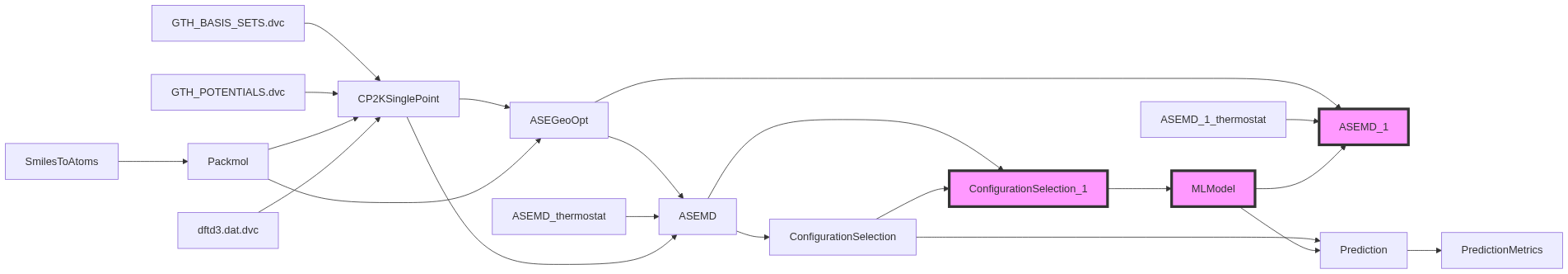
For this exercise we will only focus on the highlighted Nodes. You will make some modifications to the ML model.

In [11]:

import ipsuite as ips

Example Script¶

In the following notebook, you can see a fully prepared script for:

Generating DFT data
Selecting training and test data
Fitting a machine-learned inter-atomic potential
Deploying the potential in an MD simulation

This cell will run immediately as results of a pre-run model will be loaded. Take note of each step as you will need some of them later.

In [ ]:

mapping = ips.geometry.BarycenterMapping(data=None)
thermostat = ips.calculators.LangevinThermostat(
    temperature=300, friction=0.01, time_step=0.5
)

with ips.Project(automatic_node_names=True) as project:
    mol = ips.configuration_generation.SmilesToAtoms(smiles="O")
    
    # Create a box of atoms.
    packmol = ips.configuration_generation.Packmol(
        data=[mol.atoms], count=[10], density=997
    )
    
    # Define the CP2K calculations
    cp2k = ips.calculators.CP2KSinglePoint(
        data=packmol,
        cp2k_files=["GTH_BASIS_SETS", "GTH_POTENTIALS", "dftd3.dat"],
        cp2k_shell="cp2k_shell.psmp",
    )
    
    # Perform geometry optimization
    geopt = ips.calculators.ASEGeoOpt(
        model=cp2k,
        data=packmol.atoms,
        optimizer="BFGS",
        run_kwargs={"fmax": 0.1},
    )
    
    # Define an integrator
    md = ips.calculators.ASEMD(
        model=cp2k,
        thermostat=thermostat,
        data=geopt.atoms,
        data_id=-1,
        sampling_rate=1,
        dump_rate=1,
        steps=5000,
    )
    
    # Split data into test and train
    test_data = ips.configuration_selection.RandomSelection(
        data=md, n_configurations=250
    )
    train_data = ips.configuration_selection.RandomSelection(
        data=md,
        n_configurations=250,
        exclude_configurations=[
            test_data.selected_configurations,
        ],
    )
    
    # Define a model
    model = ips.models.GAP(data=train_data, soap={"cutoff": 3, "l_max": 5, "n_max": 5})
    
    # Use model to make some predicitons
    predictions = ips.analysis.Prediction(data=test_data, model=model)
    analysis = ips.analysis.PredictionMetrics(data=predictions)
    
    # Use model in an MD simulation.
    ml_md = ips.calculators.ASEMD(
        model=model,
        thermostat=thermostat,
        data=geopt.atoms,
        data_id=-1,
        sampling_rate=1,
        dump_rate=1,
        steps=5000,
    )

# Run all of the steps.
project.run(repro=False)

Training your own models¶

Now that you have seen what it looks like, you can start playing with your own models, but first, let's load up the previous model and see how it performed.

Download the model¶

In [ ]:

!dvc pull --quiet

Compute the RMSE scores¶

RMSE scores provide one with an idea of how far away an ML models predictions are from the underlying DFT data. In this case it has been computed for you but later, you will need to do this yourself so keep an eye on where to get the data from.

In [3]:

analysis.load()  # Required for IPSuite to run

In [ ]:

analysis.energy

In [ ]:

analysis.energy_df.iloc[:5]

The following correlation plots was also generated automatically and might help you evaluate the ML Model accuracy.

In [ ]:

from IPython.display import display, Image, display_pretty, Pretty
display(Image(filename='nodes/PredictionMetrics/plots/energy.png'))
display(Image(filename='nodes/PredictionMetrics/plots/forces.png'))

Compute the Radial Distribution Function¶

The next thing you want to do is see how well the model performed in a real MD simulation. To do so, we compare the radial distirbution function of the md run with the machine-learned potential with the underlying DFT data on which it was trained

Load the DFT DATA¶

In [ ]:

md.load()
md.atoms[:5]

Load the ML-MD Simulation Data¶

In [ ]:

ml_md.load()
ml_md.atoms[:5]

Compute the RDF¶

In [9]:

import ase
import ase.geometry.analysis
import matplotlib.pyplot as plt
import numpy as np

In [10]:

data = ase.geometry.analysis.Analysis(ml_md.atoms).get_rdf(rmax=3.0, nbins=100, elements=["H", "O"])
dft_data = ase.geometry.analysis.Analysis(md.atoms).get_rdf(rmax=3.0, nbins=100, elements=["H", "O"])

In [ ]:

fig, ax = plt.subplots()
ax.plot(np.linspace(0, 3.0, 100), np.mean(data, axis=0), label="ML PES")
ax.plot(np.linspace(0, 3.0, 100), np.mean(dft_data, axis=0), label="DFT")
ax.hlines(xmin=0, xmax=3, y=1, ls="--")
ax.set_xlabel(r"Distance r / $\AA$")
ax.set_ylabel("RDF g(r)")
ax.legend()

Fit your own ML model¶

Now that we have looked at a pretrained model, it is time train some of your own. We will create IPSuite Experiments to accomplish this.

Fit five models with data-set sizes ranging from 10, to 200 and make a plot of their RMSE scores with respect to their data-set sizes and explain what you see.

If you have lost track of all the experiments that you performed, you can use dvc exp show from the command line to view them in a tabular form.

with project.create_experiment() as exp1:
    train_data.n_configurations = 10    

with project.create_experiment() as exp2:
    ...

# copy this line to run the experiments
!dvc exp run --run-all

print(exp1[analysis.name].energy)
print(exp1[train_data.name].n_configurations)

In [33]:

# Your experiments

Deploying a Pre-Trained Model¶

You have used the GAP model up until now. For the last part we will have a look at another ML Model, called MACE https://github.com/ACEsuit/mace

For this example training a MACE model takes longer than training a GAP model. Therefore, we will look at a pretrained model that we can download.

We will save our current model and load the MACE model afterwards.

In [6]:

!git add .
!git commit -m "new ML Model"

[main 4b07b60] new ML Model
 3 files changed, 1031 insertions(+), 20 deletions(-)
 create mode 100644 .ipynb_checkpoints/main-checkpoint.ipynb

In [7]:

!git checkout mace

Branch 'mace' set up to track remote branch 'mace' from 'origin'.
Switched to a new branch 'mace'

In [ ]:

!dvc pull --quiet

The following images show the correlation plots of the MACE model. How much do they differ from your best GAP model? Copy and paste the code from the Analyse the Results section above again and evaluate your model. Because we are using MACE instead of GAP we need to change the Model via model = ips.models.MACE.from_rev(). Especially compare the RDF of the MACE model with your GAP model.

In [15]:

model = ips.models.MACE.from_rev()

In [ ]:

display(Image(filename='nodes/PredictionMetrics/plots/energy.png'))
display(Image(filename='nodes/PredictionMetrics/plots/forces.png'))

Lastly, let us scale things up a bit. With DFT we are limited to small box sizes. With our ML-Pes we can have a look at bigger boxes. We can set the repeat attribute of our ASEMD Node to increase the box size.

Perform an MD simulation for an unscaled and scaled simulation box. Compute the RDF for each simulation and compare them to one another and the DFT data you loaded at the start of the notebook. Discuss in your report what you see.

with project.create_experiment() as mace_exp1:
    # original size
    ml_md.repeat = (1, 1, 1)

with project.create_experiment() as mace_exp2:
    # 8 times the volume
    ml_md.repeat = (2, 2, 2)


project.run_exp()

mace_exp1[ml_md.name].atoms # access the atoms to print the RDF

In [ ]:

# Your code here.

Return to your model¶

These are just some lines required for IPSuite to work correctly if you want to go back to your model.

In [ ]:

!git checkout main
!dvc checkout