ETHZ: 227-0966-00L¶

Quantitative Big Imaging¶

March 19, 2019¶

Supervised Segmentation Approaches¶

Anders Kaestner¶

Reading Material¶

Overview¶

Methods
Pipelines
Classification
Regression
Segmentation

In [1]:

import seaborn as sns
import matplotlib.pyplot as plt
plt.rcParams["figure.figsize"] = (8, 8)
plt.rcParams["figure.dpi"] = 150
plt.rcParams["font.size"] = 14
plt.rcParams['font.family'] = ['sans-serif']
plt.rcParams['font.sans-serif'] = ['DejaVu Sans']
plt.style.use('ggplot')
sns.set_style("whitegrid", {'axes.grid': False})

Basic Methods Overview¶

There are a number of supervised methods we can use for

classification,
regression
and both.

Workflow of supervised methods¶

Training¶

The training phase is when the parameters of the model are learned
Used training data with ground truth.

Predicting¶

Provides responses on inputs using the trained model.
Uses new unseen data.

Basic Methods Overview¶

There are a number of methods we can use for classification, regression and both. For the simplification of the material we will not make a massive distinction between classification and regression but there are many situations where this is not appropriate. Here we cover a few basic methods, since these are important to understand as a starting point for solving difficult problems. The list is not complete and importantly Support Vector Machines are completely missing which can be a very useful tool in supervised analysis. A core idea to supervised models is they have a training phase and a predicting phase.

Training¶

The training phase is when the parameters of the model are learned and involve putting inputs into the model and updating the parameters so they better match the outputs. This is a sort-of curve fitting (with linear regression it is exactly curve fitting).

Predicting¶

The predicting phase is once the parameters have been set applying the model to new datasets. At this point the parameters are no longer adjusted or updated and the model is frozen. Generally it is not possible to tweak a model any more using new data but some approaches (most notably neural networks) are able to handle this.

Lets create some data...¶

Here we create some bivariate data 'blobs' with Gaussian distribution

In [2]:

import pandas as pd
import numpy as np
import matplotlib.pyplot as plt
from sklearn.datasets import make_blobs
%matplotlib inline

blob_data, blob_labels = make_blobs(n_samples=100,
                                    random_state=2018)
test_pts = pd.DataFrame(blob_data, columns=['x', 'y'])
test_pts['group_id'] = blob_labels
plt.scatter(test_pts.x, test_pts.y,
            c=test_pts.group_id,
            cmap='viridis')
test_pts.sample(5)

Out[2]:

	x	y	group_id
38	7.780745	-8.841535	0
22	-1.227507	1.605207	2
13	6.958921	-7.479881	0
70	7.469452	-6.328131	1
66	8.017615	-9.517988	0

Nearest Neighbor (or K Nearest Neighbors)¶

The technique is as basic as it sounds, it basically finds the nearest point to what you have put in.

In [4]:

plt.figure(figsize=[6,6])
plt.scatter(test_pts.x, test_pts.y,
            c=test_pts.group_id,
            cmap='viridis')
plt.plot(2,-2,'X',color='cornflowerblue',markersize=10,label='Point A')
plt.plot(7.7,-6.1,'o',color='darkorange',markersize=10,label='Point B')
plt.plot(8.5,-4,'P',color='deeppink',markersize=10,label='Point C')
plt.legend();

Text example¶

Training data¶

Value	1	2	3	4
Class	I	am	a	dog

Start the training¶

In [32]:

from sklearn.neighbors import KNeighborsClassifier
import numpy as np
k_class = KNeighborsClassifier(1)
k_class.fit(X=np.reshape([0, 1, 2, 3], (-1, 1)),
            y=['I', 'am', 'a', 'dog'])

Out[32]:

KNeighborsClassifier(algorithm='auto', leaf_size=30, metric='minkowski',
                     metric_params=None, n_jobs=None, n_neighbors=1, p=2,
                     weights='uniform')

Nearest neighbor predictions¶

Basic test¶

Same values as training

In [35]:

print(k_class.predict(np.reshape([0, 1, 2, 3],
                                 (-1, 1))))

['I' 'am' 'a' 'dog']

Testing with different values¶

In [36]:

print("Input 1.5 :",k_class.predict(np.reshape([1.5], (1, 1))))
print("Input 100 :",k_class.predict(np.reshape([100], (1, 1))))

Input 1.5 : ['am']
Input 100 : ['dog']

Let's come back to the blob data¶

In [37]:

import pandas as pd
import numpy as np
import matplotlib.pyplot as plt
from sklearn.datasets import make_blobs
%matplotlib inline

blob_data, blob_labels = make_blobs(n_samples=100,
                                    cluster_std=2.0,
                                    random_state=2018)
test_pts = pd.DataFrame(blob_data, columns=['x', 'y'])
test_pts['group_id'] = blob_labels
plt.scatter(test_pts.x, test_pts.y, c=test_pts.group_id, cmap='viridis')
test_pts.sample(5)

Out[37]:

	x	y	group_id
67	-2.016102	1.901388	2
51	5.225736	-8.526798	0
56	9.661421	-5.665855	1
20	3.204612	-7.015864	0
6	-0.049603	0.930626	2

Training the model using one neighbor¶

In [38]:

k_class = KNeighborsClassifier(1)
k_class.fit(test_pts[['x', 'y']], test_pts['group_id']) 

Out[38]:

KNeighborsClassifier(algorithm='auto', leaf_size=30, metric='minkowski',
                     metric_params=None, n_jobs=None, n_neighbors=1, p=2,
                     weights='uniform')

Resulting prediction map for a single neighbor¶

In [39]:

xx, yy = np.meshgrid(np.linspace(test_pts.x.min(), test_pts.x.max(), 30),np.linspace(test_pts.y.min(), test_pts.y.max(), 30),indexing='ij');
grid_pts = pd.DataFrame(dict(x=xx.ravel(), y=yy.ravel()))
grid_pts['predicted_id'] = k_class.predict(grid_pts[['x', 'y']])

fig, (ax1, ax2) = plt.subplots(1, 2, figsize=(12, 4))
ax1.scatter(test_pts.x, test_pts.y, c=test_pts.group_id, cmap='viridis'); ax1.set_title('Training Data');
ax2.scatter(grid_pts.x, grid_pts.y, c=grid_pts.predicted_id, cmap='viridis'); ax2.set_title('Testing Points');

Stabilizing Results - Increase number of neighbors¶

We can see here that the result is thrown off by single points
Prediction can be improved by using more than the nearest neighbor

In [40]:

k_class = KNeighborsClassifier(4)
k_class.fit(test_pts[['x', 'y']], test_pts['group_id'])
xx, yy = np.meshgrid(np.linspace(test_pts.x.min(), test_pts.x.max(), 30),
                     np.linspace(test_pts.y.min(), test_pts.y.max(), 30),
                     indexing='ij'
                     )
grid_pts = pd.DataFrame(dict(x=xx.ravel(), y=yy.ravel()))
grid_pts['predicted_id'] = k_class.predict(grid_pts[['x', 'y']])

fig, (ax1, ax2) = plt.subplots(1, 2, figsize=(12, 4))
ax1.scatter(test_pts.x, test_pts.y, c=test_pts.group_id, cmap='viridis'); ax1.set_title('Training Data');
ax2.scatter(grid_pts.x, grid_pts.y, c=grid_pts.predicted_id, cmap='viridis');ax2.set_title('Testing Points with 4 neighbors');

Linear Regression¶

Linear regression is a fancy-name for linear curve fitting
Fitting a line through points (sometimes in more than one dimension).
It is a very basic method,
- is easy to understand,
- interpret
- and fast to compute

We need data to fit...¶

In [8]:

from sklearn.linear_model import LinearRegression
import numpy as np
x = np.array([0, 1, 2, 3])
y = np.array([10, 20, 30, 40] )
plt.plot(x,y,'o',color='cornflowerblue'); plt.title('Training data')
l_reg = LinearRegression()
l_reg.fit(X=np.reshape(x, (-1, 1)),y=y)
print("slope: {0:0.4}, intercept: {1:0.4}".format(l_reg.coef_[0], l_reg.intercept_))

slope: 10.0, intercept: 10.0

Let's try the model on some data points¶

In [41]:

print('An array of values:',l_reg.predict(np.reshape([0, 1, 2, 3], (-1, 1))))
print('x:',-100, '=>', l_reg.predict(np.reshape([-100], (1, 1))))
print('x: ',500, '=>', l_reg.predict(np.reshape([500], (1, 1))))

---------------------------------------------------------------------------
ValueError                                Traceback (most recent call last)
<ipython-input-41-a677c3b61797> in <module>
----> 1 print('An array of values:',l_reg.predict(np.reshape([0, 1, 2, 3], (-1, 1))))
      2 print('x:',-100, '=>', l_reg.predict(np.reshape([-100], (1, 1))))
      3 print('x: ',500, '=>', l_reg.predict(np.reshape([500], (1, 1))))

~/opt/anaconda3/lib/python3.7/site-packages/sklearn/linear_model/_base.py in predict(self, X)
    223             Returns predicted values.
    224         """
--> 225         return self._decision_function(X)
    226 
    227     _preprocess_data = staticmethod(_preprocess_data)

~/opt/anaconda3/lib/python3.7/site-packages/sklearn/linear_model/_base.py in _decision_function(self, X)
    207         X = check_array(X, accept_sparse=['csr', 'csc', 'coo'])
    208         return safe_sparse_dot(X, self.coef_.T,
--> 209                                dense_output=True) + self.intercept_
    210 
    211     def predict(self, X):

~/opt/anaconda3/lib/python3.7/site-packages/sklearn/utils/extmath.py in safe_sparse_dot(a, b, dense_output)
    149             ret = np.dot(a, b)
    150     else:
--> 151         ret = a @ b
    152 
    153     if (sparse.issparse(a) and sparse.issparse(b)

ValueError: matmul: Input operand 1 has a mismatch in its core dimension 0, with gufunc signature (n?,k),(k,m?)->(n?,m?) (size 2 is different from 1)

In [42]:

from sklearn.datasets import make_blobs
import matplotlib.pyplot as plt

import numpy as np
import pandas as pd
blob_data, blob_labels = make_blobs(centers=2, n_samples=100,
                                    random_state=2018)
test_pts = pd.DataFrame(blob_data, columns=['x', 'y'])
test_pts['group_id'] = blob_labels
plt.scatter(test_pts.x, test_pts.y, c=test_pts.group_id, cmap='viridis')
test_pts.sample(5)

Out[42]:

	x	y	group_id
28	5.425799	-7.464655	0
17	8.149263	-7.057416	0
27	8.411070	-8.283136	0
15	8.715819	-4.644777	1
11	6.365924	-6.119970	1

In [43]:

l_reg = LinearRegression()
l_reg.fit(test_pts[['x', 'y']], test_pts['group_id'])
print('Slope', l_reg.coef_)
print('Offset', l_reg.intercept_)

Slope [0.04813137 0.20391973]
Offset 1.346929708594462

In [11]:

xx, yy = np.meshgrid(np.linspace(test_pts.x.min(), test_pts.x.max(), 20),
                     np.linspace(test_pts.y.min(), test_pts.y.max(), 20),
                     indexing='ij'
                     )
grid_pts = pd.DataFrame(dict(x=xx.ravel(), y=yy.ravel()))
grid_pts['predicted_id'] = l_reg.predict(grid_pts[['x', 'y']])

fig, (ax1, ax2, ax3) = plt.subplots(1, 3, figsize=(12, 4))
ax1.scatter(test_pts.x, test_pts.y, c=test_pts.group_id, cmap='viridis')
ax1.set_title('Training Data')
ax2.scatter(grid_pts.x, grid_pts.y, c=grid_pts.predicted_id, cmap='viridis')
ax2.set_title('Testing Points')
ax3.imshow(grid_pts.predicted_id.values.reshape(
    xx.shape).T[::-1], cmap='viridis')
ax3.set_title('Test Image');

Trees¶

SciKit Learn documentation on trees
Hastie et al., Elements Of Statistical Learning, 2009 Section 9.2 Trees.

In [12]:

from sklearn.tree import export_graphviz
import graphviz


def show_tree(in_tree):
    return graphviz.Source(export_graphviz(in_tree, out_file=None))

In [44]:

from sklearn.tree import DecisionTreeClassifier
import numpy as np
d_tree = DecisionTreeClassifier()
d_tree.fit(X=np.reshape([0, 1, 2, 3], (-1, 1)),
           y=[0, 1, 0, 1])

Out[44]:

DecisionTreeClassifier(ccp_alpha=0.0, class_weight=None, criterion='gini',
                       max_depth=None, max_features=None, max_leaf_nodes=None,
                       min_impurity_decrease=0.0, min_impurity_split=None,
                       min_samples_leaf=1, min_samples_split=2,
                       min_weight_fraction_leaf=0.0, presort='deprecated',
                       random_state=None, splitter='best')

In [14]:

show_tree(d_tree)

Out[14]:

In [45]:

import pandas as pd
import numpy as np
import matplotlib.pyplot as plt
from sklearn.datasets import make_blobs
%matplotlib inline

blob_data, blob_labels = make_blobs(n_samples=100,
                                    random_state=2018)
test_pts = pd.DataFrame(blob_data, columns=['x', 'y'])
test_pts['group_id'] = blob_labels
plt.figure(figsize=[15,4])
plt.subplot(1,2,1)

cell_text = []
for row in range(5):
    cell_text.append(test_pts.sample(5).iloc[row])

plt.table(cellText=cell_text, colLabels=test_pts.columns, loc='center')
plt.axis('off')

plt.subplot(1,2,2)
plt.scatter(test_pts.x, test_pts.y, c=test_pts.group_id, cmap='viridis')

Out[45]:

<matplotlib.collections.PathCollection at 0x7f9b8a1970d0>

In [16]:

d_tree = DecisionTreeClassifier()
d_tree.fit(test_pts[['x', 'y']],
           test_pts['group_id'])
show_tree(d_tree)

Out[16]:

In [17]:

xx, yy = np.meshgrid(np.linspace(test_pts.x.min(), test_pts.x.max(), 20),
                     np.linspace(test_pts.y.min(), test_pts.y.max(), 20),
                     indexing='ij'
                     )
grid_pts = pd.DataFrame(dict(x=xx.ravel(), y=yy.ravel()))
grid_pts['predicted_id'] = d_tree.predict(grid_pts[['x', 'y']])

fig, (ax1, ax2) = plt.subplots(1, 2, figsize=(12, 4))
ax1.scatter(test_pts.x, test_pts.y, c=test_pts.group_id, cmap='viridis')
ax1.set_title('Training Data')
ax2.scatter(grid_pts.x, grid_pts.y, c=grid_pts.predicted_id, cmap='viridis')
ax2.set_title('Testing Points')

Out[17]:

Text(0.5, 1.0, 'Testing Points')

Forests¶

Forests are basically the idea of taking a number of trees and bringing them together. So rather than taking a single tree to do the classification, you divide the samples and the features to make different trees and then combine the results. One of the more successful approaches is called Random Forests or as a video

In [18]:

import pandas as pd
import numpy as np
import matplotlib.pyplot as plt
from sklearn.datasets import make_blobs
%matplotlib inline

blob_data, blob_labels = make_blobs(n_samples=1000,
                                    cluster_std=3,
                                    random_state=2018)
test_pts = pd.DataFrame(blob_data, columns=['x', 'y'])
test_pts['group_id'] = blob_labels
plt.scatter(test_pts.x, test_pts.y, c=test_pts.group_id, cmap='viridis')

Out[18]:

<matplotlib.collections.PathCollection at 0x7f9b78b71590>

In [19]:

from sklearn.ensemble import RandomForestClassifier
rf_class = RandomForestClassifier(n_estimators=5, random_state=2018)
rf_class.fit(test_pts[['x', 'y']], 
            
             test_pts['group_id'])
print('Build ', len(rf_class.estimators_), 'decision trees')

Build  5 decision trees

In [20]:

show_tree(rf_class.estimators_[0])

Out[20]:

In [21]:

show_tree(rf_class.estimators_[1])

Out[21]:

In [46]:

xx, yy = np.meshgrid(np.linspace(test_pts.x.min(), test_pts.x.max(), 20),
                     np.linspace(test_pts.y.min(), test_pts.y.max(), 20),
                     indexing='ij'
                     )
grid_pts = pd.DataFrame(dict(x=xx.ravel(), y=yy.ravel()))

fig, (ax1, ax2, ax3, ax4) = plt.subplots(1, 4, figsize=(14, 3), dpi=150)
ax1.scatter(test_pts.x, test_pts.y, c=test_pts.group_id, cmap='viridis')
ax1.set_title('Training Data')
ax2.scatter(grid_pts.x, grid_pts.y, c=rf_class.predict(
    grid_pts[['x', 'y']]), cmap='viridis')
ax2.set_title('Random Forest Classifier')

ax3.scatter(grid_pts.x, grid_pts.y, c=rf_class.estimators_[
            0].predict(grid_pts[['x', 'y']]), cmap='viridis')
ax3.set_title('First Decision Tree')

ax4.scatter(grid_pts.x, grid_pts.y, c=rf_class.estimators_[
            1].predict(grid_pts[['x', 'y']]), cmap='viridis')
ax4.set_title('Second Decision Tree')

Out[46]:

Text(0.5, 1.0, 'Second Decision Tree')

Pipelines¶

We will use the idea of pipelines generically here to refer to the combination of steps that need to be performed to solve a problem.

In [22]:

%%file pipe_utils.py
from sklearn.preprocessing import FunctionTransformer
import numpy as np
from skimage.filters import laplace, gaussian, median
from skimage.util import montage as montage2d
import matplotlib.pyplot as plt



def display_data(in_ax, raw_data, show_hist):
    if (raw_data.shape[0] == 1) and (len(raw_data.shape) == 4):
        # reformat channels first
        in_data = raw_data[0].swapaxes(0, 2).swapaxes(1, 2)
    else:
        in_data = np.squeeze(raw_data)
    if len(in_data.shape) == 1:
        if show_hist:
            in_ax.hist(in_data)
        else:
            in_ax.plot(in_data, 'r.')
    elif len(in_data.shape) == 2:
        if show_hist:
            for i in range(in_data.shape[1]):
                in_ax.hist(in_data[:, i], label='Dim:{}'.format(i), alpha=0.5)
            in_ax.legend()
        else:
            if in_data.shape[1] == 2:
                in_ax.plot(in_data[:, 0], in_data[:, 1], 'r.')
            else:
                in_ax.plot(in_data, '.')
    elif len(in_data.shape) == 3:
        if show_hist:
            in_ax.hist(in_data.ravel())
        else:
            n_stack = np.stack([(x-x.mean())/x.std() for x in in_data], 0)
            in_ax.imshow(montage2d(n_stack))


def show_pipe(pipe, in_data, show_hist=False):
    m_rows = np.ceil((len(pipe.steps)+1)/3).astype(int)
    fig, t_axs = plt.subplots(m_rows, 3, figsize=(12, 5*m_rows))
    m_axs = t_axs.flatten()
    [c_ax.axis('off') for c_ax in m_axs]
    last_data = in_data
    for i, (c_ax, (step_name, step_op)) in enumerate(zip(m_axs, [('Input Data', None)]+pipe.steps), 1):
        if step_op is not None:
            try:
                last_data = step_op.transform(last_data)
            except AttributeError:
                try:
                    last_data = step_op.predict_proba(last_data)
                except AttributeError:
                    last_data = step_op.predict(last_data)

        display_data(c_ax, last_data, show_hist)
        c_ax.set_title('Step {} {}\n{}'.format(i, last_data.shape, step_name))
        c_ax.axis('on')


def flatten_func(x): return np.reshape(x, (np.shape(x)[0], -1))


flatten_step = FunctionTransformer(flatten_func, validate=False)


def px_flatten_func(in_x):
    if len(in_x.shape) == 2:
        x = np.expand_dims(in_x, -1)
    elif len(in_x.shape) == 3:
        x = in_x
    elif len(in_x.shape) == 4:
        x = in_x
    else:
        raise ValueError(
            'Cannot work with images with dimensions {}'.format(in_x.shape))
    return np.reshape(x, (-1, np.shape(x)[-1]))


px_flatten_step = FunctionTransformer(px_flatten_func, validate=False)


def add_filters(in_x, filt_func=[lambda x: gaussian(x, sigma=2),
                                 lambda x: gaussian(
                                     x, sigma=5)-gaussian(x, sigma=2),
                                 lambda x: gaussian(x, sigma=8)-gaussian(x, sigma=5)]):
    if len(in_x.shape) == 2:
        x = np.expand_dims(np.expand_dims(in_x, 0), -1)
    elif len(in_x.shape) == 3:
        x = np.expand_dims(in_x, -1)
    elif len(in_x.shape) == 4:
        x = in_x
    else:
        raise ValueError(
            'Cannot work with images with dimensions {}'.format(in_x.shape))
    n_img, x_dim, y_dim, c_dim = x.shape
    out_imgs = [x]
    for c_filt in filt_func:
        out_imgs += [np.stack([np.stack([c_filt(x[i, :, :, j])
                                         for i in range(n_img)], 0)
                               for j in range(c_dim)], -1)]

    return np.concatenate(out_imgs, -1)


filter_step = FunctionTransformer(add_filters, validate=False)


def add_xy_coord(in_x, polar=False):
    if len(in_x.shape) == 2:
        x = np.expand_dims(np.expand_dims(in_x, 0), -1)
    elif len(in_x.shape) == 3:
        x = np.expand_dims(in_x, -1)
    elif len(in_x.shape) == 4:
        x = in_x
    else:
        raise ValueError(
            'Cannot work with images with dimensions {}'.format(in_x.shape))
    n_img, x_dim, y_dim, c_dim = x.shape

    _, xx, yy, _ = np.meshgrid(np.arange(n_img),
                               np.arange(x_dim),
                               np.arange(y_dim),
                               [1],
                               indexing='ij')
    if polar:
        rr = np.sqrt(np.square(xx-xx.mean())+np.square(yy-yy.mean()))
        th = np.arctan2(yy-yy.mean(), xx-xx.mean())
        return np.concatenate([x, rr, th], -1)
    else:
        return np.concatenate([x, xx, yy], -1)


xy_step = FunctionTransformer(add_xy_coord, validate=False)
polar_step = FunctionTransformer(
    lambda x: add_xy_coord(x, polar=True), validate=False)


def fit_img_pipe(in_pipe, in_x, in_y):
    in_pipe.fit(in_x,
                px_flatten_func(in_y)[:, 0])

    def predict_func(new_x):
        x_dim, y_dim = new_x.shape[0:2]
        return in_pipe.predict(new_x).reshape((x_dim, y_dim, -1))
    return predict_func

Overwriting pipe_utils.py

In [23]:

import pandas as pd
import numpy as np
import matplotlib.pyplot as plt
from sklearn.datasets import make_blobs
%matplotlib inline


blob_data, blob_labels = make_blobs(n_samples=100,
                                    random_state=2018)
test_pts = pd.DataFrame(blob_data, columns=['x', 'y'])
test_pts['group_id'] = blob_labels

fig, (ax1, ax2) = plt.subplots(1, 2, figsize=(15, 4))
cell_text = []
for row in range(5):
    cell_text.append(test_pts.sample(5).iloc[row])

ax1.table(cellText=cell_text, colLabels=test_pts.columns, loc='center')
ax1.axis('off')

ax2.scatter(test_pts.x, test_pts.y, c=test_pts.group_id, cmap='viridis')

Out[23]:

<matplotlib.collections.PathCollection at 0x7f9baa35f190>

In [24]:

from pipe_utils import show_pipe
from sklearn.pipeline import Pipeline
from sklearn.preprocessing import RobustScaler
simple_pipe = Pipeline([('Normalize', RobustScaler())])
simple_pipe.fit(test_pts)

show_pipe(simple_pipe, test_pts.values)
show_pipe(simple_pipe, test_pts.values, show_hist=True)

In [25]:

from sklearn.preprocessing import QuantileTransformer
longer_pipe = Pipeline([('Quantile', QuantileTransformer(2)),
                        ('Normalize', RobustScaler())
                        ])
longer_pipe.fit(test_pts)

show_pipe(longer_pipe, test_pts.values)
show_pipe(longer_pipe, test_pts.values, show_hist=True)

In [26]:

from sklearn.preprocessing import PolynomialFeatures
messy_pipe = Pipeline([
    ('Normalize', RobustScaler()),
    ('PolynomialFeatures', PolynomialFeatures(2)),
])
messy_pipe.fit(test_pts)

show_pipe(messy_pipe, test_pts.values)
show_pipe(messy_pipe, test_pts.values, show_hist=True)

Classification¶

A common problem of putting images into categories.

The standard problem for this is classifying digits between 0 and 9 (MNIST).
Fundamentally a classification problem is one where we are taking a large input (images, vectors, ...) and trying to put it into a category.
- Cats, Dogs
- Cars, boats
- etc.

Lets load some images¶

Images of numbers 0 to 9
8 $\times$ 8 pixels
50 Samples

In [47]:

from sklearn.datasets import load_digits
import pandas as pd
import numpy as np
import matplotlib.pyplot as plt
from sklearn.datasets import make_blobs 
from pipe_utils import show_pipe
%matplotlib inline
digit_ds = load_digits(return_X_y=False)
img_data = digit_ds.images[:50]
digit_id = digit_ds.target[:50]
print('Image Data', img_data.shape)

Image Data (50, 8, 8)

Run a preprocessing pipline¶

Flatten images 8 $\times$ 8 $\rightarrow$ 1 $\times$ 64
Normalize (robust scaling)

In [48]:

from pipe_utils import flatten_step
from sklearn.pipeline import Pipeline
from sklearn.preprocessing import RobustScaler
digit_pipe = Pipeline([('Flatten', flatten_step),
                       ('Normalize', RobustScaler())])
digit_pipe.fit(img_data)

show_pipe(digit_pipe, img_data)
show_pipe(digit_pipe, img_data, show_hist=True)

Add a classifier¶

Add a K Nearest Neighbours classifier to the pipeline (K=1)
Run the fit

In [49]:

from sklearn.neighbors import KNeighborsClassifier

digit_class_pipe = Pipeline([('Flatten', flatten_step),
                             ('Normalize', RobustScaler()),
                             ('NearestNeighbor', KNeighborsClassifier(1))])
digit_class_pipe.fit(img_data, digit_id)

show_pipe(digit_class_pipe, img_data)

Test classifier performance¶

Let's test with traning data

In [50]:

from sklearn.metrics import accuracy_score
pred_digit = digit_class_pipe.predict(img_data)
print('{0}% accuracy'.format(100*accuracy_score(digit_id, pred_digit)))

100.0% accuracy

How about the confusion matrix?¶

In [51]:

from sklearn.metrics import confusion_matrix
import seaborn as sns
fig, ax1 = plt.subplots(1, 1, figsize=(8, 8), dpi=100)
sns.heatmap(
    confusion_matrix(digit_id, pred_digit),
    annot=True,
    fmt='d',
    ax=ax1)

Out[51]:

<matplotlib.axes._subplots.AxesSubplot at 0x7f9b7a700210>

In [52]:

from sklearn.metrics import classification_report
print(classification_report(digit_id, pred_digit))

              precision    recall  f1-score   support

           0       1.00      1.00      1.00         7
           1       1.00      1.00      1.00         5
           2       1.00      1.00      1.00         3
           3       1.00      1.00      1.00         4
           4       1.00      1.00      1.00         4
           5       1.00      1.00      1.00         7
           6       1.00      1.00      1.00         4
           7       1.00      1.00      1.00         5
           8       1.00      1.00      1.00         5
           9       1.00      1.00      1.00         6

    accuracy                           1.00        50
   macro avg       1.00      1.00      1.00        50
weighted avg       1.00      1.00      1.00        50

Wow! We've built an amazing algorithm!¶

Let's patent it! Call Google!¶

Let's try again¶

Using new, unseen data

In [53]:

test_digit = np.array([[[0.,  0.,  6., 12., 13.,  6.,  0.,  0.],
                        [0.,  6., 16.,  9., 12., 16.,  2.,  0.],
                        [0.,  7., 16.,  9., 15., 13.,  0.,  0.],
                        [0.,  0., 11., 15., 16.,  4.,  0.,  0.],
                        [0.,  0.,  0., 12., 10.,  0.,  0.,  0.],
                        [0.,  0.,  3., 16.,  4.,  0.,  0.,  0.],
                        [0.,  0.,  1., 16.,  2.,  0.,  0.,  0.],
                        [0.,  0.,  6., 11.,  0.,  0.,  0.,  0.]]])
plt.matshow(test_digit[0], cmap='bone')
print('Prediction:', digit_class_pipe.predict(test_digit))
print('Real Value:', 9)

Prediction: [7]
Real Value: 9

Training, Validation, and Testing¶

Avoid the training crime in ML¶

https://www.kdnuggets.com/2017/08/dataiku-predictive-model-holdout-cross-validation.html

Regression¶

For regression, we can see

it is very similarly to a classification
- Predicts the category
instead of trying to output discrete classes we can output on a continuous scale.
- Predicts the actual decimal number.

In [54]:

from sklearn.datasets import load_digits
import pandas as pd
import numpy as np
import matplotlib.pyplot as plt
from sklearn.datasets import make_blobs
from pipe_utils import show_pipe, flatten_step
%matplotlib inline
digit_ds = load_digits(return_X_y=False)

img_data = digit_ds.images[:50]
digit_id = digit_ds.target[:50]

valid_data = digit_ds.images[50:500]
valid_id = digit_ds.target[50:500]

In [55]:

from sklearn.neighbors import KNeighborsRegressor

digit_regress_pipe = Pipeline([('Flatten', flatten_step),
                               ('Normalize', RobustScaler()),
                               ('NearestNeighbor', KNeighborsRegressor(1))])
digit_regress_pipe.fit(img_data, digit_id)

show_pipe(digit_regress_pipe, img_data)

Assessment¶

We can't use accuracy, ROC, precision, recall or any of these factors anymore since we don't have binary / true-or-false conditions we are trying to predict. We know have to go back to some of the initial metrics we covered in the first lectures.

$$ MSE = \frac{1}{N}\sum \left(y_{predicted} - y_{actual}\right)^2 $$$$ MAE = \frac{1}{N}\sum |y_{predicted} - y_{actual}| $$

In [56]:

import seaborn as sns
fig, (ax1, ax2) = plt.subplots(1, 2, figsize=(12, 6), dpi=100)
pred_train = digit_regress_pipe.predict(img_data)
jitter = lambda x: x+0.25*np.random.uniform(-1, 1, size=x.shape)
sns.swarmplot(digit_id, jitter(pred_train), ax=ax1)
ax1.set_title('Predictions (Training)\nMSE: %2.2f MAE: %2.2f' % (np.mean(np.square(pred_train-digit_id)),
                                                                 np.mean(np.abs(pred_train-digit_id))))

pred_valid = digit_regress_pipe.predict(valid_data)
sns.swarmplot(valid_id, jitter(pred_valid), ax=ax2)
ax2.set_title('Predictions (Validation)\nMSE: %2.2f MAE: %2.2f' % (np.mean(np.square(pred_valid-valid_id)),
                                                                   np.mean(np.abs(pred_valid-valid_id))))

Out[56]:

Text(0.5, 1.0, 'Predictions (Validation)\nMSE: 7.71 MAE: 1.41')

Increasing neighbor count¶

In [57]:

digit_regress_pipe = Pipeline([('Flatten', flatten_step),
                               ('Normalize', RobustScaler()),
                               ('NearestNeighbor', KNeighborsRegressor(2))])
digit_regress_pipe.fit(img_data, digit_id)

show_pipe(digit_regress_pipe, img_data)

In [58]:

import seaborn as sns
fig, (ax1, ax2) = plt.subplots(1, 2, figsize=(12, 6), dpi=200)
pred_train = digit_regress_pipe.predict(img_data)

sns.swarmplot(digit_id, jitter(pred_train), ax=ax1)
ax1.set_title('Predictions (Training)\nMSE: %2.2f MAE: %2.2f' % (np.mean(np.square(pred_train-digit_id)),
                                                                 np.mean(np.abs(pred_train-digit_id))))

pred_valid = digit_regress_pipe.predict(valid_data)
sns.swarmplot(valid_id, jitter(pred_valid), ax=ax2)
ax2.set_title('Predictions (Validation)\nMSE: %2.2f MAE: %2.2f' % (np.mean(np.square(pred_valid-valid_id)),
                                                                   np.mean(np.abs(pred_valid-valid_id))));

Segmentation (Pixel Classification)¶

Previously¶

Predict something based on the information in the image

Single class (classification)
Values (regression)

Segmentation¶

Now we want to change problem:

instead of assigning a single class for each image,
we want a class or value for each pixel.

This requires that we restructure the problem.

Where segmentation fails: Mitochondria Segmentation in EM¶

The mitocondria are visible and humans easily spot them
Other structures have same gray levels
SNR is not ideal

A simple threshold is insufficient to finding the mitocondria structures
Other filtering techniques are unlikely to magicially fix this problem

Let's try some methods to segment the mitochondria image¶

Decision trees¶

DecisionTreeRegressor
DecisionTreeRegressor with position

Random forests¶

Random forest + KMeans
Random forest + polynomials
Random forest + Filters

Linear regression¶

Neighborhood

Nearest neighbor¶

KNeighborsRegressor

U-Net¶

Loading the mitchondria image and mask¶

First we need image data for:

Training
Validation

In [59]:

import pandas as pd
import numpy as np
import matplotlib.pyplot as plt
from skimage.io import imread
%matplotlib inline
cell_img = (imread("../common/data/em_image.png")[::2, ::2])/255.0
cell_seg = imread("../common/data/em_image_seg.png",
                  as_gray=True)[::2, ::2] > 0
np.random.seed(2018)
fig, (ax1, ax2) = plt.subplots(1, 2, figsize=(12, 8), dpi=72)
ax1.imshow(cell_img, cmap='bone'); ax1.set_title("EM image ({0}x{1})".format(cell_img.shape[0],cell_img.shape[1]))
ax2.imshow(cell_seg, cmap='bone'); ax2.set_title("Mask image ({0}x{1})".format(cell_seg.shape[0],cell_seg.shape[1]));

Training and validation data¶

We only have one image available...

Solution: Split it into two parts!

In [60]:

train_img, valid_img = cell_img[:, :256], cell_img[:, 256:]
train_mask, valid_mask = cell_seg[:, :256], cell_seg[:, 256:]

fig, ((ax1, ax2,ax3, ax4)) = plt.subplots(1, 4, figsize=(15, 5), dpi=100)
ax1.imshow(train_img, cmap='bone');  ax1.set_title('Train Image ({0}x{1})'.format(train_img.shape[0],train_img.shape[1]))
ax2.imshow(train_mask, cmap='bone'); ax2.set_title('Train Mask ({0}x{1})'.format(train_mask.shape[0],train_mask.shape[1]))

ax3.imshow(valid_img,  cmap='bone'); ax3.set_title('Validation Image ({0}x{1})'.format(valid_img.shape[0],valid_img.shape[1]))
ax4.imshow(valid_mask, cmap='bone'); ax4.set_title('Validation Mask ({0}x{1})'.format(valid_mask.shape[0],valid_mask.shape[1]))

Out[60]:

Text(0.5, 1.0, 'Validation Mask (384x256)')

Try a Regression tree¶

In [61]:

from pipe_utils import px_flatten_step, show_pipe, fit_img_pipe
from sklearn.pipeline import Pipeline
from sklearn.preprocessing import RobustScaler
from sklearn.cluster import KMeans
from sklearn.ensemble import RandomForestRegressor
from sklearn.tree import DecisionTreeRegressor

rf_seg_model = Pipeline([('Pixel Flatten', px_flatten_step),
                         ('Robust Scaling', RobustScaler()),
                         ('Decision Tree', DecisionTreeRegressor())
                         ])

pred_func = fit_img_pipe(rf_seg_model, train_img, train_mask)
show_pipe(rf_seg_model, train_img)
show_tree(rf_seg_model.steps[-1][1])

Out[61]:

In [62]:

fig, ((ax1, ax5, ax2), (ax3, ax6, ax4)) = plt.subplots(
    2, 3, figsize=(12, 8), dpi=72)
ax1.imshow(train_img, cmap='bone')
ax1.set_title('Train Image')

ax5.imshow(train_mask, cmap='viridis')
ax5.set_title('Train Mask')

ax2.imshow(pred_func(train_img)[:, :, 0],
           cmap='viridis', vmin=0, vmax=1)
ax2.set_title('Prediction Mask')

ax3.imshow(cell_img, cmap='bone')
ax3.set_title('Full Image')

ax6.imshow(cell_seg, cmap='viridis')
ax6.set_title('Full Mask')

ax4.imshow(pred_func(cell_img)[:, :, 0],
           cmap='viridis', vmin=0, vmax=1)
ax4.set_title('Prediction Mask')

Out[62]:

Text(0.5, 1.0, 'Prediction Mask')

Regression tree with position information¶

In [63]:

from pipe_utils import xy_step

rf_xyseg_model = Pipeline([('Add XY', xy_step),
                           ('Pixel Flatten', px_flatten_step),
                           ('Normalize', RobustScaler()),
                           ('DecisionTree', DecisionTreeRegressor(
                               min_samples_split=1000))
                           ])

pred_func = fit_img_pipe(rf_xyseg_model, train_img, train_mask)
show_pipe(rf_xyseg_model, train_img)
show_tree(rf_xyseg_model.steps[-1][1])

Out[63]:

Did we improve the segmentation performance?¶

In [64]:

fig, ((ax1, ax5, ax2), (ax3, ax6, ax4)) = plt.subplots(2, 3, figsize=(12, 8), dpi=72)
ax1.imshow(train_img, cmap='bone');ax1.set_title('Train Image')
ax5.imshow(train_mask, cmap='viridis'); ax5.set_title('Train Mask')
ax2.imshow(pred_func(train_img)[:, :, 0], cmap='viridis', vmin=0, vmax=1); ax2.set_title('Prediction Mask')
ax3.imshow(cell_img, cmap='bone'); ax3.set_title('Full Image')
ax6.imshow(cell_seg, cmap='viridis'); ax6.set_title('Full Mask')
ax4.imshow(pred_func(cell_img)[:, :, 0], cmap='viridis', vmin=0, vmax=1);ax4.set_title('Prediction Mask');

Combine K-Means and Random Forest Regression¶

In [65]:

from sklearn.cluster import KMeans
rf_xyseg_k_model = Pipeline([('Add XY', xy_step),
                             ('Pixel Flatten', px_flatten_step),
                             ('Normalize', RobustScaler()),
                             ('KMeans', KMeans(4)),
                             ('RandomForest', RandomForestRegressor(n_estimators=25))
                             ])

pred_func = fit_img_pipe(rf_xyseg_k_model, train_img, train_mask)
show_pipe(rf_xyseg_k_model, train_img)

In [66]:

fig, ((ax1, ax5, ax2), (ax3, ax6, ax4)) = plt.subplots(
    2, 3, figsize=(12, 8), dpi=72)
ax1.imshow(train_img, cmap='bone'); ax1.set_title('Train Image')
ax5.imshow(train_mask, cmap='viridis'); ax5.set_title('Train Mask')
ax2.imshow(pred_func(train_img)[:, :, 0], cmap='viridis', vmin=0, vmax=1); ax2.set_title('Prediction Mask')
ax3.imshow(cell_img, cmap='bone'); ax3.set_title('Full Image')
ax6.imshow(cell_seg, cmap='viridis'); ax6.set_title('Full Mask')
ax4.imshow(pred_func(cell_img)[:, :, 0], cmap='viridis', vmin=0, vmax=1); ax4.set_title('Prediction Mask');

In [67]:

from sklearn.preprocessing import PolynomialFeatures
rf_xyseg_py_model = Pipeline([('Add XY', xy_step),
                              ('Pixel Flatten', px_flatten_step),
                              ('Normalize', RobustScaler()),
                              ('Polynomial Features', PolynomialFeatures(2)),
                              ('RandomForest', RandomForestRegressor(n_estimators=25))
                              ])

pred_func = fit_img_pipe(rf_xyseg_py_model, train_img, train_mask)
show_pipe(rf_xyseg_py_model, train_img)

In [68]:

fig, ((ax1, ax5, ax2), (ax3, ax6, ax4)) = plt.subplots(
    2, 3, figsize=(12, 8), dpi=72)
ax1.imshow(train_img, cmap='bone')
ax1.set_title('Train Image')

ax5.imshow(train_mask, cmap='viridis')
ax5.set_title('Train Mask')

ax2.imshow(pred_func(train_img)[:, :, 0],
           cmap='viridis', vmin=0, vmax=1)
ax2.set_title('Prediction Mask')

ax3.imshow(cell_img, cmap='bone')
ax3.set_title('Full Image')

ax6.imshow(cell_seg, cmap='viridis')
ax6.set_title('Full Mask')

ax4.imshow(pred_func(cell_img)[:, :, 0],
           cmap='viridis', vmin=0, vmax=1)
ax4.set_title('Prediction Mask')

Out[68]:

Text(0.5, 1.0, 'Prediction Mask')

Adding Smarter Features¶

Here we add images with filters based on Gaussians

In [69]:

import scipy.stats as stats 
x=np.linspace(-25,25,200)
fig,(ax1,ax2,ax3) = plt.subplots(1,3,figsize=[15,4])
ax1.plot(x,stats.norm.pdf(x,0,2)); ax1.set_title("Gaussian $\sigma$=2");
ax2.plot(x,stats.norm.pdf(x,0,5)-stats.norm.pdf(x,0,2)), ax2.set_title("Gaussian $\sigma$=5 - Gaussian $\sigma$=2");
ax3.plot(x,stats.norm.pdf(x,0,8)-stats.norm.pdf(x,0,5)), ax3.set_title("Gaussian $\sigma$=8 - Gaussian $\sigma$=5");

Pipeline with filters¶

In [70]:

from pipe_utils import filter_step
rf_filterseg_model = Pipeline([('Filters', filter_step),
                               ('Pixel Flatten', px_flatten_step),
                               ('Normalize', RobustScaler()),
                               ('RandomForest', RandomForestRegressor(n_estimators=25))
                               ])

pred_func = fit_img_pipe(rf_filterseg_model, train_img, train_mask)
show_pipe(rf_filterseg_model, train_img)

In [71]:

fig, ((ax1, ax5, ax2), (ax3, ax6, ax4)) = plt.subplots(
    2, 3, figsize=(12, 8), dpi=72)
ax1.imshow(train_img, cmap='bone')
ax1.set_title('Train Image')

ax5.imshow(train_mask, cmap='viridis')
ax5.set_title('Train Mask')

ax2.imshow(pred_func(train_img)[:, :, 0],
           cmap='viridis', vmin=0, vmax=1)
ax2.set_title('Prediction Mask')

ax3.imshow(cell_img, cmap='bone')
ax3.set_title('Full Image')

ax6.imshow(cell_seg, cmap='viridis')
ax6.set_title('Full Mask')

ax4.imshow(pred_func(cell_img)[:, :, 0],
           cmap='viridis', vmin=0, vmax=1)
ax4.set_title('Prediction Mask')

Out[71]:

Text(0.5, 1.0, 'Prediction Mask')

Using the Neighborhood¶

We can also include the whole neighborhood

shifting the image in x and y by $\pm$1 pixel.
Gives nine feature images

For the first example we will then use linear regression so we can see the exact coefficients that result.

In [72]:

from sklearn.preprocessing import FunctionTransformer


def add_neighborhood(in_x, x_steps=3, y_steps=3):
    if len(in_x.shape) == 2:
        x = np.expand_dims(np.expand_dims(in_x, 0), -1)
    elif len(in_x.shape) == 3:
        x = np.expand_dims(in_x, -1)
    elif len(in_x.shape) == 4:
        x = in_x
    else:
        raise ValueError(
            'Cannot work with images with dimensions {}'.format(in_x.shape))
    n_img, x_dim, y_dim, c_dim = x.shape
    out_imgs = []
    for i in range(-x_steps, x_steps+1):
        for j in range(-y_steps, y_steps+1):
            out_imgs += [np.roll(np.roll(x,
                                         axis=1, shift=i),
                                 axis=2,
                                 shift=j)]
    return np.concatenate(out_imgs, -1)


def neighbor_step(x_steps=3, y_steps=3):
    return FunctionTransformer(
        lambda x: add_neighborhood(x, x_steps, y_steps),
        validate=False)

In [73]:

from sklearn.linear_model import LinearRegression
linreg_neighborseg_model = Pipeline([('Neighbors', neighbor_step(1, 1)),
                               ('Pixel Flatten', px_flatten_step),
                               ('Linear Regression', LinearRegression())
                               ])

pred_func = fit_img_pipe(linreg_neighborseg_model, train_img, train_mask)
show_pipe(linreg_neighborseg_model, train_img)

In [74]:

fig, ((ax1, ax5, ax2), (ax3, ax6, ax4)) = plt.subplots(
    2, 3, figsize=(12, 8), dpi=72)
ax1.imshow(train_img, cmap='bone')
ax1.set_title('Train Image')

ax5.imshow(train_mask, cmap='viridis')
ax5.set_title('Train Mask')

ax2.imshow(pred_func(train_img)[:, :, 0],
           cmap='viridis', vmin=0, vmax=1)
ax2.set_title('Prediction Mask')

ax3.imshow(cell_img, cmap='bone')
ax3.set_title('Full Image')

ax6.imshow(cell_seg, cmap='viridis')
ax6.set_title('Full Mask')

ax4.imshow(pred_func(cell_img)[:, :, 0],
           cmap='viridis', vmin=0, vmax=1)
ax4.set_title('Prediction Mask')

Out[74]:

Text(0.5, 1.0, 'Prediction Mask')

Why Linear Regression?¶

We choose linear regression so we could get easily understood coefficients.

The model fits $\vec{m}$ and $b$ to the $\vec{x}_{i,j}$ points in the image $I(i,j)$ to match the $y_{i,j}$ output in the segmentation as closely as possible $$ y_{i,j} = \vec{m}\cdot\vec{x_{i,j}}+b $$ For a 3x3 cases this looks like $$ \vec{x}_{i,j} = \left[I(i-1,j-1), I(i-1, j), I(i-1, j+1) \dots I(i+1,j-1), I(i+1, j), I(i+1, j+1)\right] $$

In [76]:

m = linreg_neighborseg_model.steps[-1][1].coef_
b = linreg_neighborseg_model.steps[-1][1].intercept_
print('M: [{:0.4}, {:0.4}, {:0.4}, {:0.4}, \033[1m{:0.4}\033[0m, {:0.4}, {:0.4}, {:0.4}, {:0.4}]'.format(m[0],m[1],m[2],m[3],m[4],m[5],m[6],m[7],m[8]))
print('b: {:0.4}'.format(b))

M: [-0.1501, -0.05296, -0.1412, -0.02355, 0.06657, -0.04512, -0.1015, -0.03607, -0.1819]
b: 0.4213

Convolution¶

The steps we have here make up a convolution and so what we have effectively done is use linear regression to learn which coefficients we should use in a convolutional kernel to get the best results

In [77]:

from scipy.ndimage import convolve
m_mat = m.reshape((3, 3)).T
fig, (ax1, ax2, ax3, ax4) = plt.subplots(1, 4, figsize=(16, 4))
sns.heatmap(m_mat,
            annot=True,
            ax=ax1, fmt='2.2f',
            vmin=-m_mat.std(),
            vmax=m_mat.std())
ax1.set_title(r'Kernel $\vec{m}$')
ax2.imshow(cell_img)
ax2.set_title('Input Image')
ax2.axis('off')

ax3.imshow(convolve(cell_img, m_mat)+b,
           vmin=0,
           vmax=1,
           cmap='viridis')
ax3.set_title('Post Convolution Image')
ax3.axis('off')

ax4.imshow(pred_func(cell_img)[:, :, 0],
           cmap='viridis', vmin=0, vmax=1)
ax4.set_title('Predicted from Linear Model')
ax4.axis('off')

Out[77]:

(-0.5, 511.5, 383.5, -0.5)

Nearest Neighbor¶

We can also use the neighborhood and nearest neighbor, this means for each pixel and its surrounds we find the pixel in the training set that looks most similar

In [78]:

nn_neighborseg_model = Pipeline([('Neighbors', neighbor_step(1, 1)),
                               ('Pixel Flatten', px_flatten_step),
                               ('Normalize', RobustScaler()),
                               ('NearestNeighbor', KNeighborsRegressor(n_neighbors=1))
                               ])

pred_func = fit_img_pipe(nn_neighborseg_model, train_img, train_mask)
show_pipe(nn_neighborseg_model, train_img)

In [79]:

fig, ((ax1, ax5, ax2), (ax3, ax6, ax4)) = plt.subplots(
    2, 3, figsize=(12, 8), dpi=72)
ax1.imshow(train_img, cmap='bone')
ax1.set_title('Train Image')

ax5.imshow(train_mask, cmap='viridis')
ax5.set_title('Train Mask')

ax2.imshow(pred_func(train_img)[:, :, 0],
           cmap='viridis', vmin=0, vmax=1)
ax2.set_title('Prediction Mask')

ax3.imshow(cell_img, cmap='bone')
ax3.set_title('Full Image')

ax6.imshow(cell_seg, cmap='viridis')
ax6.set_title('Full Mask')

ax4.imshow(pred_func(cell_img)[:, :, 0],
           cmap='viridis', vmin=0, vmax=1)
ax4.set_title('Prediction Mask')

Out[79]:

Text(0.5, 1.0, 'Prediction Mask')

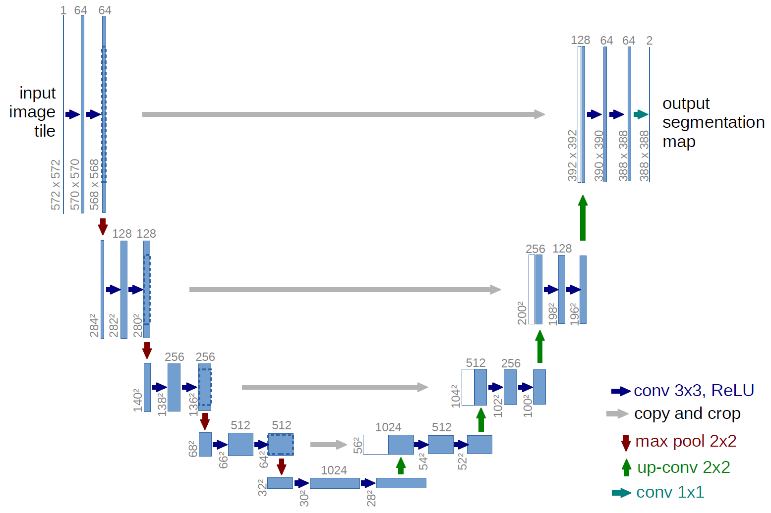
U-Net¶

The last approach we will briefly cover is the idea of U-Net a landmark paper from 2015 that dominates MICCAI submissions and contest winners today. A nice overview of the techniques is presented by Vladimir Iglovikov a winner of a recent Kaggle competition on masking images of cars slides

U-Net Diagram

In [80]:

from keras.models import Model
from keras.layers import Input, Conv2D, MaxPool2D, UpSampling2D, concatenate
from IPython.display import SVG
from keras.utils.vis_utils import model_to_dot
base_depth = 32
in_img = Input((None, None, 1), name='Image_Input')
lay_1 = Conv2D(base_depth, kernel_size=(3, 3), padding='same')(in_img)
lay_2 = Conv2D(base_depth, kernel_size=(3, 3), padding='same')(lay_1)
lay_3 = MaxPool2D((2, 2))(lay_2)
lay_4 = Conv2D(base_depth*2, kernel_size=(3, 3), padding='same')(lay_3)
lay_5 = Conv2D(base_depth*2, kernel_size=(3, 3), padding='same')(lay_4)
lay_6 = MaxPool2D((2, 2))(lay_5)
lay_7 = Conv2D(base_depth*4, kernel_size=(3, 3), padding='same')(lay_6)
lay_8 = Conv2D(base_depth*4, kernel_size=(3, 3), padding='same')(lay_7)
lay_9 = UpSampling2D((2, 2))(lay_8)
lay_10 = concatenate([lay_5, lay_9])
lay_11 = Conv2D(base_depth*2, kernel_size=(3, 3), padding='same')(lay_10)
lay_12 = Conv2D(base_depth*2, kernel_size=(3, 3), padding='same')(lay_11)
lay_13 = UpSampling2D((2, 2))(lay_12)
lay_14 = concatenate([lay_2, lay_13])
lay_15 = Conv2D(base_depth, kernel_size=(3, 3), padding='same')(lay_14)
lay_16 = Conv2D(base_depth, kernel_size=(3, 3), padding='same')(lay_15)
lay_17 = Conv2D(1, kernel_size=(1, 1), padding='same',
                activation='sigmoid')(lay_16)
t_unet = Model(inputs=[in_img], outputs=[lay_17], name='SmallUNET')
dot_mod = model_to_dot(t_unet, show_shapes=True, show_layer_names=False)
dot_mod.set_rankdir('UD')
SVG(dot_mod.create_svg())

Out[80]:

In [81]:

t_unet.summary()

Model: "SmallUNET"
__________________________________________________________________________________________________
Layer (type)                    Output Shape         Param #     Connected to                     
==================================================================================================
Image_Input (InputLayer)        (None, None, None, 1 0                                            
__________________________________________________________________________________________________
conv2d_12 (Conv2D)              (None, None, None, 3 320         Image_Input[0][0]                
__________________________________________________________________________________________________
conv2d_13 (Conv2D)              (None, None, None, 3 9248        conv2d_12[0][0]                  
__________________________________________________________________________________________________
max_pooling2d_3 (MaxPooling2D)  (None, None, None, 3 0           conv2d_13[0][0]                  
__________________________________________________________________________________________________
conv2d_14 (Conv2D)              (None, None, None, 6 18496       max_pooling2d_3[0][0]            
__________________________________________________________________________________________________
conv2d_15 (Conv2D)              (None, None, None, 6 36928       conv2d_14[0][0]                  
__________________________________________________________________________________________________
max_pooling2d_4 (MaxPooling2D)  (None, None, None, 6 0           conv2d_15[0][0]                  
__________________________________________________________________________________________________
conv2d_16 (Conv2D)              (None, None, None, 1 73856       max_pooling2d_4[0][0]            
__________________________________________________________________________________________________
conv2d_17 (Conv2D)              (None, None, None, 1 147584      conv2d_16[0][0]                  
__________________________________________________________________________________________________
up_sampling2d_3 (UpSampling2D)  (None, None, None, 1 0           conv2d_17[0][0]                  
__________________________________________________________________________________________________
concatenate_3 (Concatenate)     (None, None, None, 1 0           conv2d_15[0][0]                  
                                                                 up_sampling2d_3[0][0]            
__________________________________________________________________________________________________
conv2d_18 (Conv2D)              (None, None, None, 6 110656      concatenate_3[0][0]              
__________________________________________________________________________________________________
conv2d_19 (Conv2D)              (None, None, None, 6 36928       conv2d_18[0][0]                  
__________________________________________________________________________________________________
up_sampling2d_4 (UpSampling2D)  (None, None, None, 6 0           conv2d_19[0][0]                  
__________________________________________________________________________________________________
concatenate_4 (Concatenate)     (None, None, None, 9 0           conv2d_13[0][0]                  
                                                                 up_sampling2d_4[0][0]            
__________________________________________________________________________________________________
conv2d_20 (Conv2D)              (None, None, None, 3 27680       concatenate_4[0][0]              
__________________________________________________________________________________________________
conv2d_21 (Conv2D)              (None, None, None, 3 9248        conv2d_20[0][0]                  
__________________________________________________________________________________________________
conv2d_22 (Conv2D)              (None, None, None, 1 33          conv2d_21[0][0]                  
==================================================================================================
Total params: 470,977
Trainable params: 470,977
Non-trainable params: 0
__________________________________________________________________________________________________

New training data¶

Smaller training image (to save time)

In [82]:

import pandas as pd
import numpy as np
import matplotlib.pyplot as plt
from skimage.io import imread
%matplotlib inline
cell_img = (imread("../common/data/em_image.png")[::2, ::2])/255.0
cell_seg = imread("../common/data/em_image_seg.png",
                  as_gray=True)[::2, ::2] > 0
train_img, valid_img = cell_img[:256, 50:250], cell_img[:, 256:]
train_mask, valid_mask = cell_seg[:256, 50:250], cell_seg[:, 256:]
# add channels and sample dimensions
def prep_img(x, n=1): return (
    prep_mask(x, n=n)-train_img.mean())/train_img.std()


def prep_mask(x, n=1): return np.stack([np.expand_dims(x, -1)]*n, 0)


print('Training', train_img.shape, train_mask.shape)
print('Validation Data', valid_img.shape, valid_mask.shape)
fig, ((ax1, ax2), (ax3, ax4)) = plt.subplots(2, 2, figsize=(8, 8), dpi=72)
ax1.imshow(train_img, cmap='bone')
ax1.set_title('Train Image')
ax2.imshow(train_mask, cmap='bone')
ax2.set_title('Train Mask')

ax3.imshow(valid_img, cmap='bone')
ax3.set_title('Validation Image')
ax4.imshow(valid_mask, cmap='bone')
ax4.set_title('Validation Mask')

Training (256, 200) (256, 200)
Validation Data (384, 256) (384, 256)

Out[82]:

Text(0.5, 1.0, 'Validation Mask')

Results from Untrained Model¶

We can make predictions with an untrained model (default parameters)
but we clearly do not expect them to be very good

In [83]:

fig, m_axs = plt.subplots(2, 3,
                          figsize=(18, 8), dpi=150)
for c_ax in m_axs.flatten():
    c_ax.axis('off')
((ax1, ax2, _), (ax3, ax4, ax5)) = m_axs
ax1.imshow(train_img, cmap='bone')
ax1.set_title('Train Image')
ax2.imshow(train_mask, cmap='viridis')
ax2.set_title('Train Mask')

ax3.imshow(cell_seg, cmap='bone')
ax3.set_title('Full Image')

unet_pred = t_unet.predict(prep_img(cell_img))[0, :, :, 0]
ax4.imshow(unet_pred,
           cmap='viridis', vmin=0, vmax=1)
ax4.set_title('Predicted Segmentation')

ax5.imshow(cell_seg,
           cmap='viridis')
ax5.set_title('Ground Truth')

Out[83]:

Text(0.5, 1.0, 'Ground Truth')

A general note on the following demo¶

This is a very bad way to train a model;

the loss function is poorly chosen,
the optimizer can be improved the learning rate can be changed,
the training and validation data should not come from the same sample (and definitely not the same measurement).

The goal is to be aware of these techniques and have a feeling for how they can work for complex problems

Training conditions¶

Loss function - MAE
Optimizer - Stochastic Gradient Decent
20 Epochs (training iterations)
Metrics
1. Binary accuracy (percentage of pixels correct classified)

$$BA=\frac{1}{N}\sum_i(f_i==g_i)$$

2. Mean absulute error

Another popular metric is the Dice score $$DSC=\frac{2|X \cap Y|}{|X|+|Y|}=\frac{2\,TP}{2TP+FP+FN}$$

Let's train the model¶

In [84]:

from keras.optimizers import SGD
t_unet.compile(
    # we use a simple loss metric of mean-squared error to optimize
    loss='mse',
    # we use stochastic gradient descent to optimize
    optimizer=SGD(lr=0.05),
    # we keep track of the number of pixels correctly classified and the mean absolute error as well
    metrics=['binary_accuracy', 'mae']
)

loss_history = t_unet.fit(prep_img(train_img, n=5),
                          prep_mask(train_mask, n=5),
                          validation_data=(prep_img(valid_img),
                                           prep_mask(valid_mask)),
                          epochs=20)

Train on 5 samples, validate on 1 samples
Epoch 1/20
5/5 [==============================] - 6s 1s/step - loss: 0.3796 - binary_accuracy: 0.1811 - mae: 0.6062 - val_loss: 0.0752 - val_binary_accuracy: 0.8984 - val_mae: 0.1842
Epoch 2/20
5/5 [==============================] - 4s 767ms/step - loss: 0.0875 - binary_accuracy: 0.8876 - mae: 0.2152 - val_loss: 0.0677 - val_binary_accuracy: 0.8980 - val_mae: 0.1648
Epoch 3/20
5/5 [==============================] - 4s 744ms/step - loss: 0.0797 - binary_accuracy: 0.8867 - mae: 0.2001 - val_loss: 0.0630 - val_binary_accuracy: 0.8975 - val_mae: 0.1535
Epoch 4/20
5/5 [==============================] - 4s 806ms/step - loss: 0.0747 - binary_accuracy: 0.8874 - mae: 0.1908 - val_loss: 0.0602 - val_binary_accuracy: 0.9030 - val_mae: 0.1447
Epoch 5/20
5/5 [==============================] - 4s 750ms/step - loss: 0.0715 - binary_accuracy: 0.8943 - mae: 0.1822 - val_loss: 0.0586 - val_binary_accuracy: 0.9068 - val_mae: 0.1375
Epoch 6/20
5/5 [==============================] - 4s 722ms/step - loss: 0.0693 - binary_accuracy: 0.9000 - mae: 0.1743 - val_loss: 0.0575 - val_binary_accuracy: 0.9092 - val_mae: 0.1318
Epoch 7/20
5/5 [==============================] - 4s 739ms/step - loss: 0.0677 - binary_accuracy: 0.9033 - mae: 0.1674 - val_loss: 0.0569 - val_binary_accuracy: 0.9113 - val_mae: 0.1273
Epoch 8/20
5/5 [==============================] - 4s 732ms/step - loss: 0.0665 - binary_accuracy: 0.9063 - mae: 0.1618 - val_loss: 0.0564 - val_binary_accuracy: 0.9134 - val_mae: 0.1236
Epoch 9/20
5/5 [==============================] - 4s 717ms/step - loss: 0.0655 - binary_accuracy: 0.9086 - mae: 0.1570 - val_loss: 0.0561 - val_binary_accuracy: 0.9147 - val_mae: 0.1206
Epoch 10/20
5/5 [==============================] - 4s 746ms/step - loss: 0.0647 - binary_accuracy: 0.9103 - mae: 0.1530 - val_loss: 0.0558 - val_binary_accuracy: 0.9157 - val_mae: 0.1181
Epoch 11/20
5/5 [==============================] - 5s 936ms/step - loss: 0.0640 - binary_accuracy: 0.9118 - mae: 0.1495 - val_loss: 0.0557 - val_binary_accuracy: 0.9167 - val_mae: 0.1160
Epoch 12/20
5/5 [==============================] - 4s 856ms/step - loss: 0.0634 - binary_accuracy: 0.9131 - mae: 0.1465 - val_loss: 0.0555 - val_binary_accuracy: 0.9174 - val_mae: 0.1142
Epoch 13/20
5/5 [==============================] - 4s 782ms/step - loss: 0.0629 - binary_accuracy: 0.9140 - mae: 0.1438 - val_loss: 0.0555 - val_binary_accuracy: 0.9177 - val_mae: 0.1126
Epoch 14/20
5/5 [==============================] - 4s 725ms/step - loss: 0.0624 - binary_accuracy: 0.9149 - mae: 0.1414 - val_loss: 0.0554 - val_binary_accuracy: 0.9182 - val_mae: 0.1113
Epoch 15/20
5/5 [==============================] - 4s 734ms/step - loss: 0.0619 - binary_accuracy: 0.9159 - mae: 0.1392 - val_loss: 0.0554 - val_binary_accuracy: 0.9186 - val_mae: 0.1101
Epoch 16/20
5/5 [==============================] - 4s 707ms/step - loss: 0.0615 - binary_accuracy: 0.9169 - mae: 0.1373 - val_loss: 0.0554 - val_binary_accuracy: 0.9190 - val_mae: 0.1090
Epoch 17/20
5/5 [==============================] - 4s 831ms/step - loss: 0.0611 - binary_accuracy: 0.9177 - mae: 0.1355 - val_loss: 0.0554 - val_binary_accuracy: 0.9193 - val_mae: 0.1080
Epoch 18/20
5/5 [==============================] - 4s 766ms/step - loss: 0.0607 - binary_accuracy: 0.9184 - mae: 0.1339 - val_loss: 0.0554 - val_binary_accuracy: 0.9194 - val_mae: 0.1072
Epoch 19/20
5/5 [==============================] - 4s 794ms/step - loss: 0.0603 - binary_accuracy: 0.9190 - mae: 0.1323 - val_loss: 0.0555 - val_binary_accuracy: 0.9196 - val_mae: 0.1064
Epoch 20/20
5/5 [==============================] - 5s 930ms/step - loss: 0.0600 - binary_accuracy: 0.9198 - mae: 0.1309 - val_loss: 0.0555 - val_binary_accuracy: 0.9196 - val_mae: 0.1057

In [85]:

fig, (ax1, ax2) = plt.subplots(1, 2,
                               figsize=(20, 7))
ax1.plot(loss_history.epoch,
         loss_history.history['mae'], 'r-', label='Training')
ax1.plot(loss_history.epoch,
         loss_history.history['val_mae'], 'b-', label='Validation')
ax1.set_title('Mean Absolute Error')
ax1.legend()

ax2.plot(loss_history.epoch,
         100*np.array(loss_history.history['binary_accuracy']), 'r-', label='Training')
ax2.plot(loss_history.epoch,
         100*np.array(loss_history.history['val_binary_accuracy']), 'b-', label='Validation')
ax2.set_title('Classification Accuracy (%)')
ax2.legend()

Out[85]:

<matplotlib.legend.Legend at 0x7f9b8a018a10>

In [86]:

fig, m_axs = plt.subplots(2, 3,
                          figsize=(18, 8), dpi=150)
for c_ax in m_axs.flatten():
    c_ax.axis('off')
((ax1, ax15, ax2), (ax3, ax4, ax5)) = m_axs
ax1.imshow(train_img, cmap='bone')
ax1.set_title('Train Image')
ax15.imshow(t_unet.predict(prep_img(train_img))[0, :, :, 0],
            cmap='viridis', vmin=0, vmax=1)
ax15.set_title('Predicted Training')
ax2.imshow(train_mask, cmap='viridis')
ax2.set_title('Train Mask')

ax3.imshow(cell_img, cmap='bone')
ax3.set_title('Full Image')
unet_pred = t_unet.predict(prep_img(cell_img))[0, :, :, 0]
ax4.imshow(unet_pred,
           cmap='viridis', vmin=0, vmax=1)
ax4.set_title('Predicted Segmentation')

ax5.imshow(cell_seg,
           cmap='viridis')
ax5.set_title('Ground Truth')

Out[86]:

Text(0.5, 1.0, 'Ground Truth')

Overfitting¶

Having a model with 470,000 free parameters means that it is quite easy to overfit the model by training for too long.

Overfitting is when:

The model has gotten very good at the training data
but hasn't generalized to other kinds of problems

Consequence: The model starts to perform worse on regions that aren't exactly the same as the training.

In [87]:

t_unet.compile(
    # we use a simple loss metric of mean-squared error to optimize
    loss='mse',
    # we use stochastic gradient descent to optimize
    optimizer=SGD(lr=0.3),
    # we keep track of the number of pixels correctly classified and the mean absolute error as well
    metrics=['binary_accuracy', 'mae']
)

loss_history = t_unet.fit(prep_img(train_img),
                          prep_mask(train_mask),
                          validation_data=(prep_img(valid_img),
                                           prep_mask(valid_mask)),
                          epochs=5)

Train on 1 samples, validate on 1 samples
Epoch 1/5
1/1 [==============================] - 2s 2s/step - loss: 0.0596 - binary_accuracy: 0.9206 - mae: 0.1296 - val_loss: 0.0560 - val_binary_accuracy: 0.9206 - val_mae: 0.1021
Epoch 2/5
1/1 [==============================] - 1s 1s/step - loss: 0.0577 - binary_accuracy: 0.9242 - mae: 0.1223 - val_loss: 0.0569 - val_binary_accuracy: 0.9191 - val_mae: 0.0999
Epoch 3/5
1/1 [==============================] - 1s 1s/step - loss: 0.0562 - binary_accuracy: 0.9260 - mae: 0.1164 - val_loss: 0.0576 - val_binary_accuracy: 0.9253 - val_mae: 0.1001
Epoch 4/5
1/1 [==============================] - 1s 1s/step - loss: 0.0618 - binary_accuracy: 0.9192 - mae: 0.1233 - val_loss: 0.1251 - val_binary_accuracy: 0.8679 - val_mae: 0.1503
Epoch 5/5
1/1 [==============================] - 1s 1s/step - loss: 0.1192 - binary_accuracy: 0.8774 - mae: 0.1330 - val_loss: 0.0986 - val_binary_accuracy: 0.8985 - val_mae: 0.1022

In [88]:

fig, (ax1, ax2) = plt.subplots(1, 2,
                               figsize=(20, 7))
ax1.plot(loss_history.epoch,
         loss_history.history['mae'], 'r-', label='Training')
ax1.plot(loss_history.epoch,
         loss_history.history['val_mae'], 'b-', label='Validation')
ax1.set_title('Mean Absolute Error')
ax1.legend()

ax2.plot(loss_history.epoch,
         100*np.array(loss_history.history['binary_accuracy']), 'r-', label='Training')
ax2.plot(loss_history.epoch,
         100*np.array(loss_history.history['val_binary_accuracy']), 'b-', label='Validation')
ax2.set_title('Classification Accuracy (%)')
ax2.legend()

Out[88]:

<matplotlib.legend.Legend at 0x7f9bad78ee50>

In [89]:

fig, m_axs = plt.subplots(2, 3,
                          figsize=(18, 8), dpi=150)
for c_ax in m_axs.flatten():
    c_ax.axis('off')
((ax1, ax15, ax2), (ax3, ax4, ax5)) = m_axs
ax1.imshow(train_img, cmap='bone')
ax1.set_title('Train Image')
ax15.imshow(t_unet.predict(prep_img(train_img))[0, :, :, 0],
            cmap='viridis', vmin=0, vmax=1)
ax15.set_title('Predicted Training')
ax2.imshow(train_mask, cmap='viridis')
ax2.set_title('Train Mask')

ax3.imshow(cell_img, cmap='bone')
ax3.set_title('Full Image')
unet_pred = t_unet.predict(prep_img(cell_img))[0, :, :, 0]
ax4.imshow(unet_pred,
           cmap='viridis', vmin=0, vmax=1)
ax4.set_title('Predicted Segmentation')

ax5.imshow(cell_seg,
           cmap='viridis')
ax5.set_title('Ground Truth');

Summary¶

Concepts of supervised segmentation
Supervised Classification
Classification vs. Segmentation
- Nearest neighbour
- Trees
- Random Forests
Regression vs Classification
Training, vali
Deep learning

In [ ]: