PyAutoGalaxy
PyAutoGalaxy is software for analysing the morphologies and structures of large multi-wavelength galaxy samples:
This notebook gives an overview of PyAutoGalaxy's features and API.
Lets first import autogalaxy, its plotting module and the other libraries we'll need.
%matplotlib inline

import autogalaxy as ag
import autogalaxy.plot as aplt

import matplotlib.pyplot as plt
from os import path
Galaxies
First, we illustrate galaxy structure calculations in PyAutoGalaxy by creating an an image of a galaxy.
To describe the emission of light, PyAutoGalaxy uses Grid2D data structures, which are two-dimensional
Cartesian grids of (y,x) coordinates.
Below, we make and plot a uniform Cartesian grid:
grid = ag.Grid2D.uniform(
    shape_native=(150, 150),
    pixel_scales=0.05,  # <- The pixel-scale describes the conversion from pixel units to arc-seconds.
)

grid_plotter = aplt.Grid2DPlotter(grid=grid)
grid_plotter.figure_2d()

Our aim is to create an image of the structures that make up a galaxy.
We therefore need analytic functions representing a galaxy's light. For this, PyAutoGalaxy uses Profile
objects, for example an ellipical sersic LightProfile object which represents a light distribution:
sersic_light_profile = ag.lp.Sersic(
    centre=(0.0, 0.0),
    ell_comps=(0.2, 0.1),
    intensity=0.005,
    effective_radius=2.0,
    sersic_index=4.0,
)
By passing this profile the Grid2D, we can evaluate the light emitted at every (y,x) coordinate on the Grid2D and
create an image of the LightProfile.
image = sersic_light_profile.image_2d_from(grid=grid)

plt.imshow(image.native) # The use of 'native' is described at the start of the HowToGalaxy tutorials.
<matplotlib.image.AxesImage at 0x7f38fed1f520>

The PyAutoGalaxy plot module provides methods for plotting objects and their properties, like the image of
a LightProfile.
Note how, unlike the matplotlib method above, this figure is displayed with axis units of arc-seconds, a colorbar, labels, a title, etc. The PyAutoGalaxy plot module takes care of all the heavy lifting that comes with making figures!
light_profile_plotter = aplt.LightProfilePlotter(
    light_profile=sersic_light_profile, grid=grid
)
light_profile_plotter.figures_2d(image=True)

In PyAutoGalaxy, a Galaxy object is a collection of LightProfile objects at a given redshift.
The code below creates two galaxies representing a galaxy merger.
galaxy_0 = ag.Galaxy(
    redshift=0.5, light=sersic_light_profile,
)

exponential_light_profile = ag.lp.Exponential(
    centre=(0.7, 0.6),
    ell_comps=(0.1, 0.0),
    intensity=0.1,
    effective_radius=0.5
)

galaxy_1 = ag.Galaxy(redshift=1.0, light=exponential_light_profile)
We can use a GalaxyPlotter to plot the properties of the galaxies.
galaxy_0_plotter = aplt.GalaxyPlotter(galaxy=galaxy_0, grid=grid)
galaxy_0_plotter.figures_2d(image=True)

galaxy_1_plotter = aplt.GalaxyPlotter(galaxy=galaxy_1, grid=grid)
galaxy_1_plotter.figures_2d(image=True)


By passing these Galaxy objects to a Plane, PyAutoGalaxy uses the galaxy redshifts to group them.
plane = ag.Plane(
    galaxies=[galaxy_0, galaxy_1],
)

image = plane.image_2d_from(grid=grid)

plane_plotter = aplt.PlanePlotter(plane=plane, grid=grid)
plane_plotter.figures_2d(image=True)

All of the objects introduced above are extensible. Galaxy objects can take many Profile's and Plane's
many Galaxy's.
Lets create a Plane with 2 galaxies which are merging, with one merger having multiple star forming clumps.
galaxy_0 = ag.Galaxy(
    redshift=0.5,
    bulge=ag.lp.Sersic(
        centre=(0.0, 0.0),
        ell_comps=ag.convert.ell_comps_from(axis_ratio=0.9, angle=45.0),
        intensity=0.2,
        effective_radius=0.8,
        sersic_index=4.0,
    ),
    disk=ag.lp.Exponential(
        centre=(0.0, 0.0),
        ell_comps=ag.convert.ell_comps_from(axis_ratio=0.7, angle=30.0),
        intensity=0.1,
        effective_radius=1.6,
    ),
    clump_0=ag.lp.Sersic(centre=(1.0, 1.0), intensity=0.5, effective_radius=0.2),
    clump_1=ag.lp.Sersic(centre=(0.5, 0.8), intensity=0.5, effective_radius=0.2),
    clump_2=ag.lp.Sersic(centre=(-1.0, -0.7), intensity=0.5, effective_radius=0.2),
    clump_3=ag.lp.Sersic(centre=(-1.0, 0.4), intensity=0.5, effective_radius=0.2),
)

galaxy_1 = ag.Galaxy(
    redshift=0.5,
    bulge=ag.lp.Sersic(
        centre=(0.0, 1.0),
        ell_comps=(0.0, 0.1),
        intensity=0.1,
        effective_radius=0.6,
        sersic_index=3.0,
    ),
)

plane = ag.Plane(galaxies=[galaxy_0, galaxy_1])

plane_plotter = aplt.PlanePlotter(plane=plane, grid=grid)
plane_plotter.figures_2d(image=True)

Chapter 1 of the HowToGalaxy Jupyter notebook lectures gives new users a full run through of galaxy calculations with PyAutoGalaxy and introduces those not familiar with galaxy structure to the core theory.
A more detailed overview of these calculations can also be found in notebooks/overview/overview_1_galaxies.ipynb.
Galaxy Modeling
Galaxy modeling is the process of taking data of a galaxy (e.g. imaging data from the Hubble Space Telescope or
interferometer data from ALMA) and fitting it with a galaxy model, to determine the LightProfile's
that best represent the observed galaxy.
Galaxy modeling uses the probabilistic programming language PyAutoFit, an open-source project that allows complex model fitting techniques to be straightforwardly integrated into scientific modeling software. Check it out if you are interested in developing your own software to perform advanced model-fitting!
We import PyAutoFit separately to PyAutoGalaxy
import autofit as af
In this example, we consider simple simulated Hubble Space Telescope imaging of a galaxy.
First, lets load this imaging dataset and plot it.
dataset_name = "simple"
dataset_path = path.join("dataset", "imaging", dataset_name)

dataset = ag.Imaging.from_fits(
    data_path=path.join(dataset_path, "image.fits"),
    psf_path=path.join(dataset_path, "psf.fits"),
    noise_map_path=path.join(dataset_path, "noise_map.fits"),
    pixel_scales=0.1,
)

dataset_plotter = aplt.ImagingPlotter(dataset=dataset)
dataset_plotter.figures_2d(data=True)

We next mask the dataset, to remove the exterior regions of the image that do not contain emission from the galaxy.
Note how when we plot the Imaging below, the figure now zooms into the masked region.
mask = ag.Mask2D.circular(
    shape_native=dataset.shape_native,
    pixel_scales=dataset.pixel_scales,
    radius=3.0
)

dataset = dataset.apply_mask(mask=mask)

dataset_plotter = aplt.ImagingPlotter(dataset=dataset)
dataset_plotter.figures_2d(data=True)
2022-02-13 14:02:39,127 - autoarray.dataset.imaging - INFO - IMAGING - Data masked, contains a total of 11281 image-pixels

We now compose the galaxy model that we fit to the data using Model objects. These behave analogously to the Galaxy,
LightProfile objects above, however their parameters are not specified and are instead determined by a fitting
procedure.
We will fit our galaxy data with two galaxies:
- The galaxy's bulge is a parametric
Sersicbulge. - The galaxy's disk is a parametric
Exponentialdisk.
The redshift of the galaxy is fixed to 0.5.
galaxy_model = af.Model(
    ag.Galaxy, redshift=0.5, bulge=ag.lp.Sersic, disk=ag.lp.Exponential
)
By printing the Model's we see that each parameters has a prior associated with it, which is used by the
model-fitting procedure to fit the model.
print(galaxy_model)
We input the galaxy model above into a Collection, which is the model we will fit.
Note how we could easily extend this object to compose more complex models containing many galaxies.
model = af.Collection(galaxies=af.Collection(galaxy=galaxy_model))
The info attribute shows the model information in a more readable format:
print(model.info)
We now choose the 'non-linear search', which is the fitting method used to determine the set of LightProfile
parameters that best-fit our data.
In this example we use nautilus, a nested sampling algorithm that in our experience has proven very effective at galaxy modeling.
search = af.Nautilus(name="introduction")
2022-02-13 14:02:39,604 - autofit.non_linear.abstract_search - INFO - Creating search
To perform the model-fit, we create an AnalysisImaging object which contains the log_likelihood_function that the
non-linear search calls to fit the galaxy model to the data.
analysis = ag.AnalysisImaging(dataset=dataset)
To perform the model-fit we pass the model and analysis to the search's fit method. This will output results (e.g., Nautilus samples, model parameters, visualization) to your computer's storage device.
However, the galaxy modeling of this system takes 10-20 minutes. Therefore, to save time in this introduction, we have
commented out the fit function below so you can skip through to the next section of the notebook. Feel free to
uncomment the code and run the galaxy modeling yourself!
Once a model-fit is running, PyAutoGalaxy outputs the results of the search to storage device on-the-fly. This includes galaxy model parameter estimates with errors non-linear samples and the visualization of the best-fit galaxy model inferred by the search so far.
# result = search.fit(model=model, analysis=analysis)
The animation below shows a slide-show of the galaxy modeling procedure. Many galaxy models are fitted to the data over and over, gradually improving the quality of the fit to the data and looking more and more like the observed image.
NOTE, the animation of a non-linear search shown below is for a strong gravitational lens using PyAutoGalaxy's child project PyAutoGalaxy. Updating the animation to show a galaxy model-fit is on the PyAutoGalaxy to-do list!
We can see that initial models give a poor fit to the data but gradually improve (increasing the likelihood) as more iterations are performed.
.. image:: https://github.com/Jammy2211/auto_files/blob/main/lensmodel.gif?raw=true :width: 600

Credit: Amy Etherington
The fit returns a Result object, which contains the best-fit Plane and FitImaging as well as the full
posterior information of the non-linear search, including all parameter samples, log likelihood values and tools to
compute the errors on the galaxy model.
Chapter 2 of the HowToGalaxy Jupyter notebook lectures gives new users a full run through of galaxy modeling, including a primer on Bayesian statistics, how a non-linear search works and effective strategies for fitting data of a galaxy.
More examples can be found in the notebooks/overview and notebooks/imaging/modeling packages.
Simulating Galaxies
PyAutoGalaxy provides tool for simulating galaxy data-sets, which can be used to test galaxy modeling pipelines and train neural networks to recognise and analyse images of galaxies.
Simulating galaxy images uses a SimulatorImaging object, which models the process that an instrument like the
Hubble Space Telescope goes through observe a galaxy. This includes accounting for the exposure time to
determine the signal-to-noise of the data, accounting for diffraction of the observed light by the telescope optics
and accounting for the background sky in the exposure which acts as a source of noise.
psf = ag.Kernel2D.from_gaussian(shape_native=(11, 11), sigma=0.1, pixel_scales=dataset.pixel_scales)

simulator = ag.SimulatorImaging(
    exposure_time=300.0, background_sky_level=1.0, psf=psf, add_poisson_noise=True
)
Once we have a simulator, we can use it to create an imaging dataset which consists of an image, noise-map and Point Spread Function (PSF) by passing it a plane and grid.
This uses the plane above to create the image of the galaxy and then add the effects that occur during data acquisition.
dataset = simulator.via_plane_from(plane=plane, grid=grid)
By plotting a subplot of the Imaging dataset, we can see this object includes the observed image of the galaxy
(which has had noise and other instrumental effects added to it) as well as a noise-map and PSF:
dataset_plotter = aplt.ImagingPlotter(dataset=dataset)
dataset_plotter.subplot_dataset()

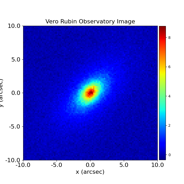
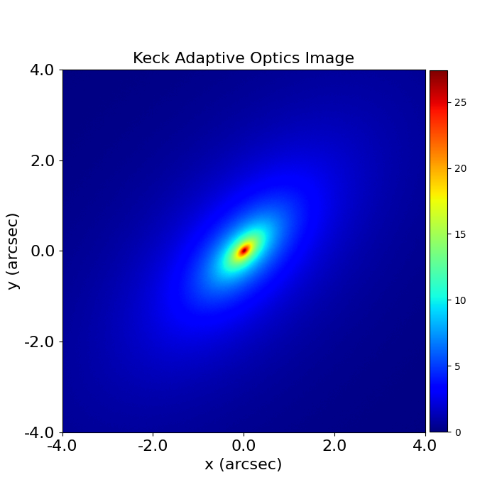
The folder notebooks/imaging/simulators includes many example notebooks for simulating galaxies with a range
of different physical properties as well as creating imaging datasets representative of a variety of telescopes
(e.g. Hubble, Euclid).
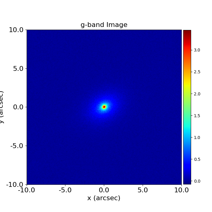
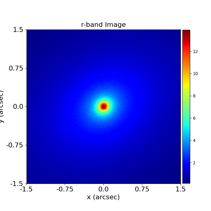
Below, we show what a galaxy observation looks like for the lowest resolution instrument in these examples (the Vera Rubin Observatory) and highest resolution instrument (Keck Adaptive Optics).
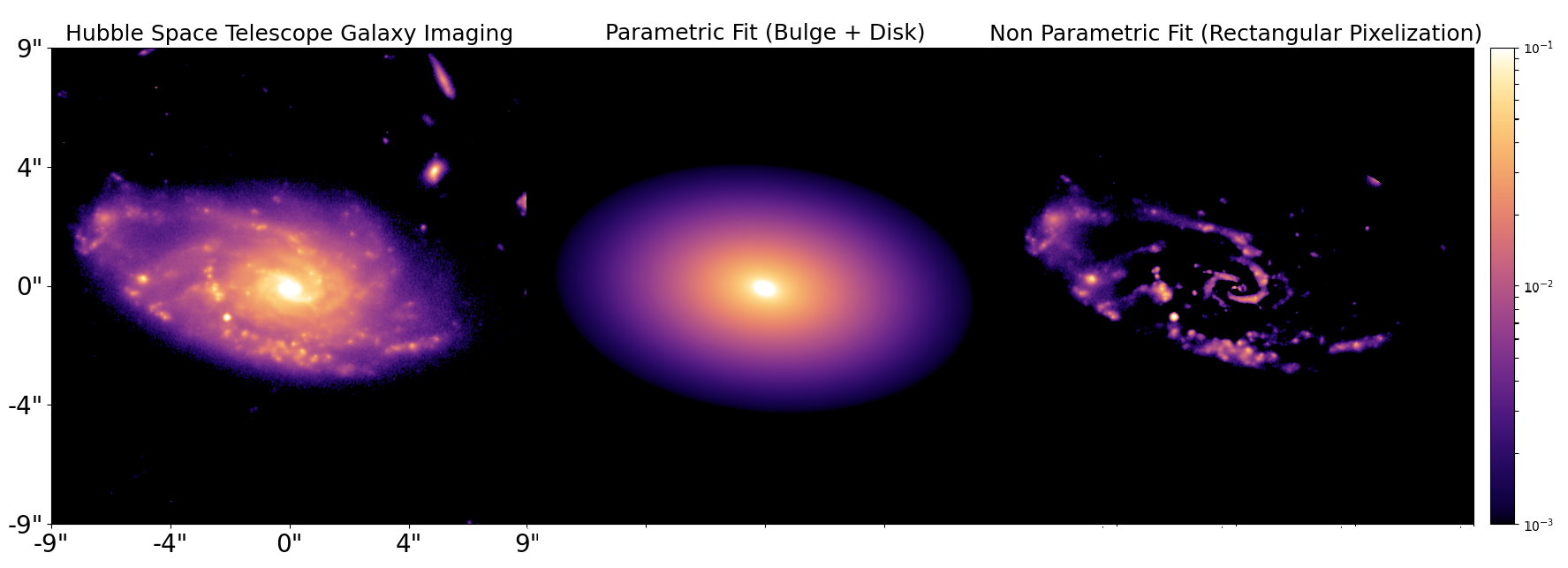
Non Parametric Models
Non parametric models reconstruct the galaxy's light on a pixel-grid. Unlike LightProfile's, they are able to
reconstruct the light of non-symmetric, irregular and clumpy sources.
The image below shows a non parametric of a galaxy observed in the Hubble Ultra Deep Field. Its bulge and disk are fitted using light profiles, whereas its asymmetric and irregular spiral arm features are fitted using the non parametric rectangular pixel-grid:
A complete overview of non parametric models can be found
at notebooks/overview/overview_5_pixelizations.ipynb. Chapter 4 of the HowToGalaxy lectures
describes non parametric models in detail and teaches users how they can be used to perform galaxy modeling.
Interferometry
PyAutoGalaxy supports modeling of interferometer data from submillimeter and radio observatories:
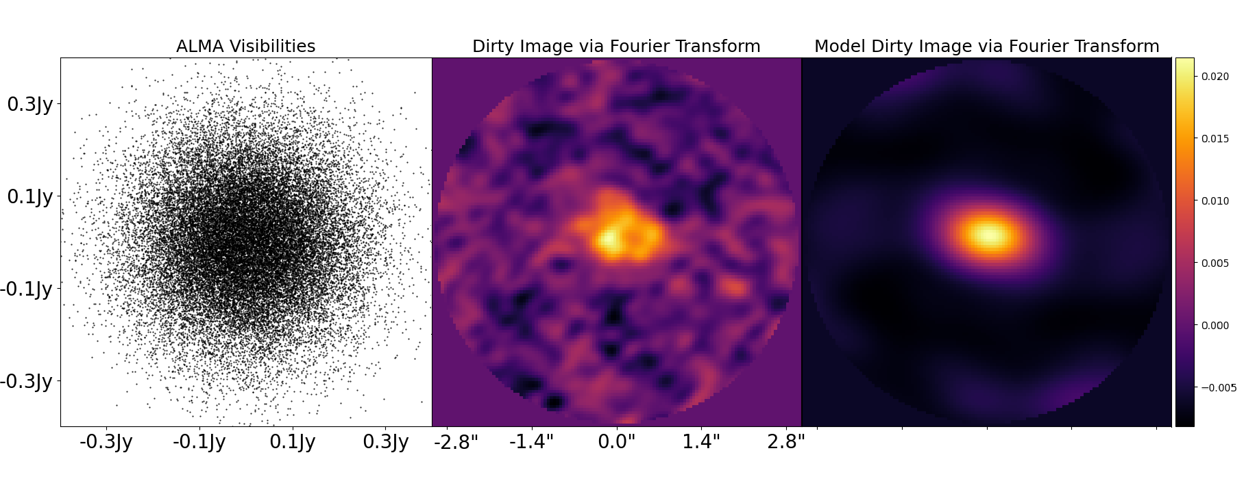
Visibilities data is fitted directly in the uv-plane, circumventing issues that arise when fitting a dirty image such as correlated noise. This uses the non-uniform fast fourier transform algorithm PyNUFFT to efficiently map the galaxy model images to the uv-plane.
Given the irregular and clumpy nature of submm / radio sources, non parametric models are a powerful tool for modeling interferometer datasets. This would be a slow process, however PyAutoGalaxy* uses the linear algebra library PyLops to ensure visibilities fitting is efficient, even for datasets consisting of tens of millions of visibilities.
An overview of interferometer analysis is given in notebooks/overview/overview_6_interferometer.ipynb and
the autogalaxy_workspace/*/interferometer package has example scripts for simulating datasets and galaxy
modeling.
Multi-Wavelength
PyAutoGalaxy supports multi-wavelength modeling of imaging datasets observed at different colors and combining these with interferometer data.
The appearance of the galaxy changes as a function of wavelength, therefore multi-wavelength galaxy modeling makes it easier to deblend the emission of different components in a galaxy (e.g a bulge and disk) and offers more information to constrain the galaxy model.
An overview of multi-wavelength analysis is given in notebooks/overview/overview_7_mutli_wavelength.ipynb and
the autogalaxy_workspace/*/multi package has example scripts for simulating datasets and galaxy modeling.
Congratulations, you've completed the PyAutoGalaxy overview!
So, What Next?
We recommend that new users start with the HowToGalaxy Jupyter notebook lectures, which provide a detailed description of the PyAutoGalaxy API and teach new users how to approach galaxy analysis, modeling and use the features described above.
You can install PyAutoGalaxy on your system and clone the autogalaxy_workspace and howtogalaxy tutorials
following the instructions on our readthedocs:
https://pyautogalaxy.readthedocs.io/en/latest/installation/overview.html
Alternatively, you can begin the tutorials on this Binder by going to the
folder notebooks/howtogalaxy/chapter_1_introduction at the following
link https://mybinder.org/v2/gh/Jammy2211/autogalaxy_workspace/HEAD
If you want to dive straight into a certain feature, example scripts for the following tasks can be found in the
following folders of the autogalaxy_workspace:
notebooks/overview: A more detailed overview of PyAutoGalaxy's features .notebooks/imaging/modeling: Example scripts for fitting a galaxy model to CCD imaging data (e.g. HST).notebooks/imaging/preprocessA Preprocessing guide for preparing your CCD dataset for PyAutoGalaxy.notebooks/imaging/simulators: Simulating CCD imaging data.notebooks/results: Tutorials explaining how to use theResultobject returned after galaxy modeling.notebooks/interferometer: Interferometer modeling and simulations.
Examples describing advanced PyAutoGalaxy features are also located throughout the autogalaxy_workspace (many are
in packages named advanced). We advise that new users omit these packages until familiar with the software:
notebooks/multi: Multi-wavelength modeling and simulations.notebooks/database: Database tools for loading and analysing the results of large-scale galaxy model fits.notebooks/imaging/advanced/chaining: Advanced modeling scripts which chain together multiple non-linear searches.