Salt polygons are caused by convection
Authors: Jana Lasser (1, 2, 3), Joanna M. Nield (4), Marcel Ernst (1), Volker Karius (5), Giles F.S. Wiggs (6), Lucas Goehring (7)
- Max Planck Institute for Dynamics and Self-Organization Göttingen
- Complexity Science Hub Vienna
- Medical University Vienna, Center for Medical Statistics, Informatics and Intelligent Systems
- Geography and Environmental Science, University of Southampton
- Geowissenschaftliches Zentrum, Georg-August-University
- Aeolian Geomorphology, University of Oxford
- School of Science and Technology, Nottingham Trent University
Table of contents 
- Abstract
- Introduction
- Model of subsurface convection
- Instability and scale selection
- Figure 4: Surface pattern scan
- [Figure 5: Pattern length scales from field, experiment, simulations
- Direct evidence for convection
- Discussion and conclusion
- Methods
- Supplementary information
- References
Abstract 
From fairy circles to patterned ground and columnar joints, natural patterns spontaneously appear in many complex geophysical settings. Here, we shed light on the origins of polygonally patterned crusts of salt playa and salt pans. These beautifully regular features, approximately a meter in diameter, are found worldwide and are fundamentally important to the transport of salt and dust in arid regions. We show that they are consistent with the surface expression of buoyancy-driven convection in the porous soil beneath a salt crust. By combining quantitative results from direct field observations, analogue experiments, linear stability theory, and numerical simulations, we further determine the conditions under which salt polygons should form, as well as how their characteristic size emerges.
Introduction 
Salt deserts are amongst the most inhospitable places of our planet. Their otherworldly shapes inspire the imagination (e.g. Star Wars desert planet Crait, or the million tourists annually visiting Death Valley, and are an important drive of climate processes [1]. The immediately prominent feature of such landscapes (Fig. 1) is a characteristic tiling of polygons, formed by ridges in the salt-encrusted surface. These patterns decorate salt pans around the world, including Salar de Uyuni in Chile, Chott el Djerid in Tunisia [2], Badwater Basin in California and the periphery of the Dead Sea -- always expressing the same size of about one meter.
Salt crusts are dynamic over months to years [3, 4, 5, 6], and couple to other environmental processes. Wind over crust creates dust, the emission of which forms a significant proportion of the Earth's global atmospheric dust production [1, 7] and of mineral transport to the oceans [8]. As one example, dust from the surface of the dry Owens Lake has posed a major health problem for people living downwind of the lake [9, 10], and the site is the centre of a decades-long, intense remediation effort. Salt crusts also modify evaporation and heat flux from the playa surface [11], and hence the critical water and energy balances of fragile environments.
Research on salt pans has typically focused on either the dynamics of their complex subsurface flows [12, 13, 14, 15, 16] or their crusts, without considering how these features could interact. Crust patterns have been attributed to buckling or wrinkling as expanding areas of crust collide [17, 18, 3], or to surface cracks [19, 20, 21, 22, 4]. For example, a model of crust patterns developing from contraction cracks in mud is given by Krinsley whereas Christiansen provides a quantitative model based on buckling, and most subsequent discussion reiterates these ideas. However, for such mechanical instabilities the expected feature size is a few times the thickness of the cracking [19, 23, 24, 25], or buckling [26, 27] layer. As well, buckling is known to favour parallel wrinkles rather than closed polygons [26, 27]. Salt playa crusts vary in thickness from sub-centimeter to meters [19, 3, 4], which cannot itself explain the consistent polygon diameters of 1--2$\,$m. Similarly, there is no clear reason why preexisting mud-cracks, surface roughness or other heterogeneities would appear worldwide at the same length-scale and arrangement. For example, at Owens Lake we observed crusts 1--20 cm thick, desiccation cracks in crust-free mud of $\sim$10 cm spacing and intermittent buckling of crust (see Supplemental Movie) with wavelengths of $\sim$2 cm and parallel rather than polygonal features. While salt precipitation may take advantage of any such pre-existing surface structures, none of these can adequately explain the patterns and scales observed in the crust polygons.
Here we show that by instead considering the surface of a salt playa jointly with its subsurface flows, the origins, dynamics, length-scale and shape of the polygonal patterns in salt crusts can be apprehended. Specifically, by combining theoretical analysis, numerical simulations, analogue experiments and field observations, we show that density-driven convective dynamics will lead to heterogeneity in the horizontal salinity distribution of evaporating groundwater, at the same scale as the observed polygons. These convective cells can act to template the position of polygons, setting their size and shape. For example, we will show how salt ridges should naturally develop over descending plumes of dense salty groundwater, where faster salt precipitation will be expected, and demonstrate such co-location in the field.
The salt polygons at Owens Lake (Fig. 1 B) have a typical pattern in a well-studied and controlled landscape; their summary also introduces our modelling assumptions and main field site. This dry, terminal saline lake has an aquifer that extends from the near-surface to $>$150$\,$m depth [28]. The groundwater carries dissolved salts [29, 10], which collect in an evaporite pan of about 300 km$^2$ [1, 28]. Efforts to control dust emission from the lake-bed involve shallow flooding [30], vegetation [31], gravel cover and crust growth [32]. As shown in the online supplementary movie S1, after a flooding event the soil is saturated with water, which evaporates leaving behind salts that crystallize into a continuous crust, covered by a network of ridges.
Figure 1: Typical salt polygon patterns 
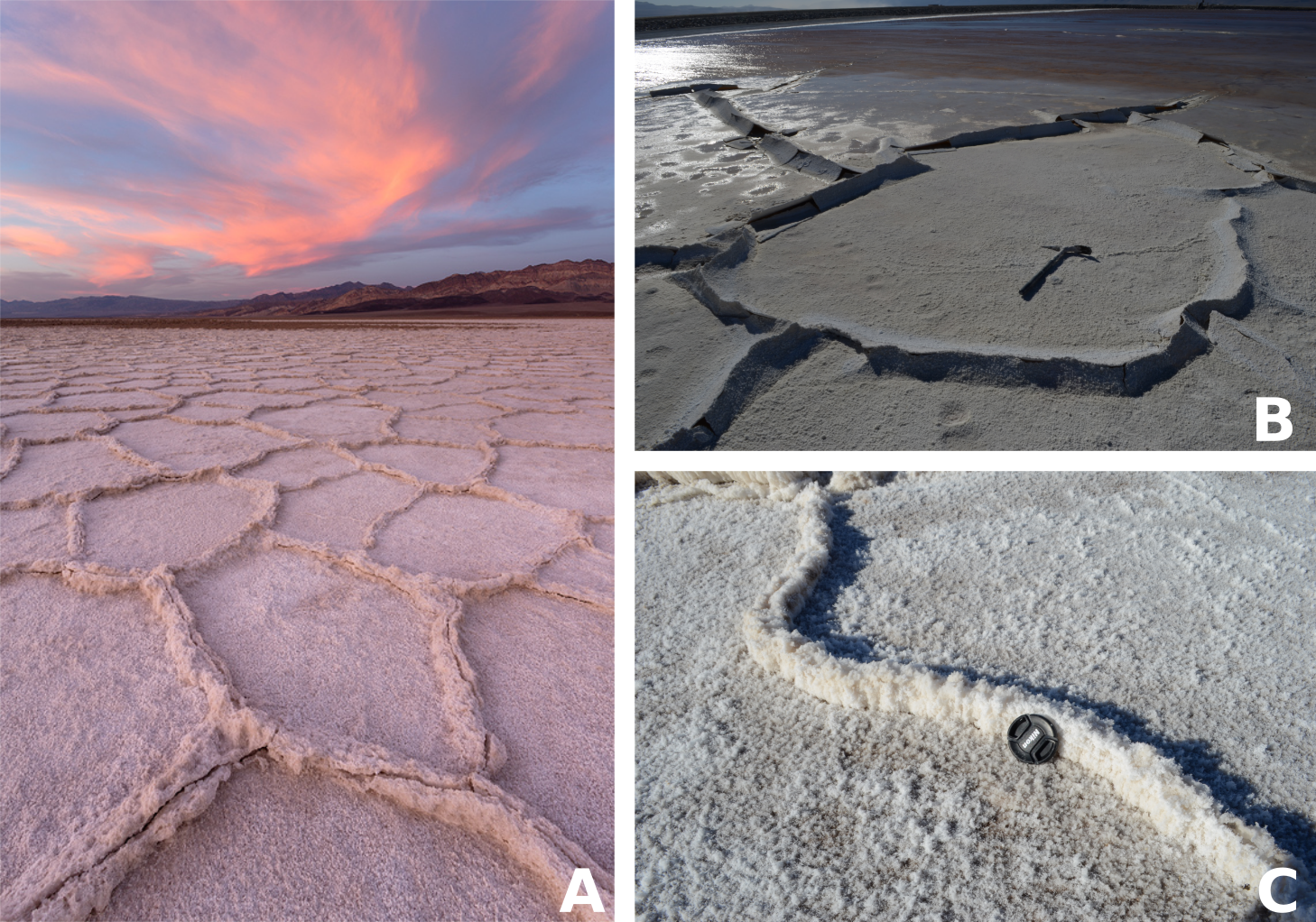
Figure 1: Typical salt polygon patterns at A, C Badwater Basin in Death Valley and B, Owens Lake, California (image A courtesy Sarah Marino).
Model of subsurface convection 
We consider the coupling of surface salt patterns to subsurface flows, as visualised in Fig. 2. Specifically, we treat fluid and salt transport in a saturated porous medium, driven by surface evaporation and fed from below by a reservoir of water with some background salinity. The aquifer is deep, compared to the diameter of the salt polygons, and any corresponding near-surface dynamics. This system will naturally develop a salinity gradient below the surface, which can become unstable to convective overturning [13, 14, 15, 16]. To determine whether field conditions will support such a buoyancy-driven convective instability, we start from mass and momentum balances, as are used to describe thermal [13] or solutal [15, 33] convection in porous media. We then perform a linear stability analysis to give the criteria for convection, and will confirm this instability via simulations, experiments and field observations.
Figure 2: Model of subsurface convection 
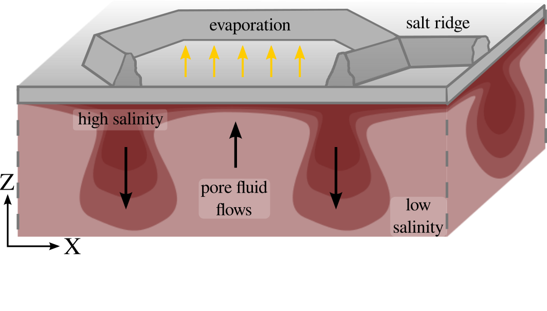
Figure 2: Proposed dynamics of patterned salt crusts. Evaporation leaves the near-surface fluid enriched in salt, and heavier than the fluid beneath it. This drives convection, with downwellings of high salinity pore fluid co-localized with surface ridges. The dominant fluid motions are shown by the black arrows, and the water salinity is indicated by the colour contours. At downwellings, the weak salt gradients in the groundwater enhance salt precipitation/crust growth, leading to ridges; at upwelling plumes the stronger gradients favour diffusive over advective transport, and crust growth is slower.
We model the volumetric flux $\boldsymbol{q}$ of a fluid driven by pressure $p$ through a porous medium of constant uniform porosity $\phi$ and permeability $\kappa$. The fluid has a viscosity $\mu$ and carries dissolved salt, whose diffusivity $D$ is corrected for the presence of different ions as well as tortuosity (see Methods). Using the Boussinesq approximation, buoyancy is generated by a variable fluid density $\rho = \rho_b+S\Delta\rho$, where $\rho_b$ is the density of the reservoir fluid, and $\rho_b +\Delta\rho$ is that of the top boundary; the relative salinity $S$ linearly mediates between the two limits. The model consists of the continuity equation for incompressible fluid flow, Darcy's law and an advection-diffusion equation for salt transport:
\begin{align} \mathrm{(1)}\quad & \boldsymbol{\nabla} \cdot \boldsymbol{q} = 0 \\ \mathrm{(2)}\quad & \boldsymbol{q} = -\frac{\kappa}{\mu}\left[ \nabla (p + \rho_b g z) + S \Delta \rho g\hat{\boldsymbol{z}}\right]\\ \mathrm{(3)}\quad & \phi\frac{\partial S}{\partial t} = \phi D\nabla^2 S - \boldsymbol{q} \cdot \nabla S\, \end{align} where $g$ is the acceleration due to gravity, and $\hat{\boldsymbol{z}}$ is an upward-pointing unit vector.
Taking the average evaporation rate $E$ as the natural velocity scale for the system, we set the characteristic length and time as $L = \phi D/E$ and $T = \phi^2D/E^2$, respectively. Non-dimensionalization of Eqs. 1-3 then gives
\begin{align} \mathrm{(4)} \quad & \boldsymbol{\nabla} \cdot \boldsymbol{U} = 0\label{eq:continuity}\\ \mathrm{(5)} \quad & \boldsymbol{U} = - \nabla P - \text{Ra} S\hat{Z}\label{eq:darcy_flow}\\ \mathrm{(6)} \quad & \frac{\partial S}{\partial \tau} = \nabla^2 S - \boldsymbol{U} \cdot \nabla S\label{eq:advection_diffusion}\; \end{align} \end{linenomath} with dimensionless velocity $\boldsymbol{U}=\boldsymbol{q}/E$, time $\tau = t/T$, vertical position $Z = {zE}/{\phi D}$ and a pressure $P = \frac{\kappa}{\phi \mu D}(p+\rho_b g z)$. This system of equations is governed by the Rayleigh number \begin{linenomath} \begin{align} \mathrm{(7)} \quad & \text{Ra} = \frac{\kappa \Delta \rho g}{ \mu E}.\label{eq:rayleigh} \end{align}
At the upper surface of the soil, $Z = 0$, we match the vertical water flux to the evaporation rate. The presence of a salt crust sets $S = 1$ there. However, the rate at which salt is added to this surface ($1-\partial S / \partial Z$, following the definition of salt flux, $S\vec{U} - \nabla S$, in Eq. (6) must allow for its transport by both advection and diffusion. As sketched in Fig. 2, this will lead to faster salt precipitation above any convective downwellings, which we argue gives rise to ridges there.
A steady-state solution to Eqs. (4) – (6), $S = \exp(-zE/\phi D)$, represents a salt-rich layer of pore fluid lying just below the salt crust, and a balance between advection and diffusion. This is unstable beyond some critical Rayleigh number, $\mathrm{Ra}_\mathrm{c}$, which depends on the boundary conditions [12, 13, 34, 35]. For constant through-flow at the surface, as expected in the field, $\mathrm{Ra}_\mathrm{c}=14.35$ for the onset of an instability that leads to down-welling plumes of high salinity [13]. Between $\mathrm{Ra} = 5.66$ and $\mathrm{Ra}_\mathrm{c}$ the fixed solution may also be unstable to finite amplitude perturbations [13, 14]. The neutral stability curve and most unstable mode of convection (see [36] for derivation) are shown in Fig. 3 below. At $\mathrm{Ra}_\mathrm{c}$ the critical wavenumber, $a_\mathrm{c}=0.76$, corresponds to a wavelength of about 1-2 m, under typical field conditions.
Figure 3: Neutral stability & most unstable mode from theory 
Imports
# imports
import numpy as np
import pandas as pd
from scipy.optimize import curve_fit
import matplotlib.pyplot as plt
import matplotlib as mpl
from matplotlib.font_manager import FontProperties
from mpl_toolkits.axes_grid1 import make_axes_locatable
from scipy.io import loadmat
from PIL import Image
import os
from ipywidgets import widgets, interactive
import warnings
warnings.filterwarnings("ignore")
Plot settings
# color codes used throughout the document
red = '#CA3542'
blue = '#27647B'
yellow = '#EBA631'
orange = '#DA5526'
purple = '#d489f6'
green = '#3c8562'
grey = '#849FAD'

# color map used throughout the document
cmap_C = plt.get_cmap('inferno_r')
# load data calculated by mathematica from the semi-analytical theory
# the data table contains a column for the wavenumber a and one for
# the Rayleigh number Ra
unstable_mode = pd.read_csv('data/most_unstable_mode.csv')
neutral_curve = pd.read_csv('data/neutral_curve.csv')
neutral_curve.head()
| a | Ra | |
|---|---|---|
| 0 | 0.010061 | 7585.209381 |
| 1 | 0.010067 | 7576.132500 |
| 2 | 0.010074 | 7567.072099 |
| 3 | 0.010080 | 7558.028138 |
| 4 | 0.010086 | 7549.000576 |
# plot the neutral stability curve and the most unstable mode
fig, ax = plt.subplots(1,1,figsize=(10,6))

ax.plot(neutral_curve['a'], neutral_curve['Ra'], color='k', \
       label='neutral stability')
ax.plot(unstable_mode['a'], unstable_mode['Ra'],'--',color=grey,\
       label='most unstable mode')

# set the y-axis to a logarithmic scale to better visuazlize
# the overall curve
ax.set_yscale('log')
ax.set_xlim([0,8])
ax.set_ylabel('Rayleigh number Ra')
ax.set_xlabel('wavenumber $a = 2\\pi/\\Lambda$')
ax.legend(loc=1,framealpha=0.9);

Figure 3: Characterising the convective instability. Stability diagram of porous media convection in salt pans. The neutral stability curve (black line) is the theoretical boundary above which an evaporating stratified pore fluid is unstable to perturbations of wavenumber $a$. Here the most unstable mode (dashed line) gives a prediction of the initial convective wavelength, and its dependence on Ra.
Instability and scale selection 
To determine the Rayleigh numbers relevant to field conditions, and to thus evaluate if they should lead to convection and an associated pattern of crust precipitation, we measured the relevant parameters at sites in Owens Lake (CA), Badwater Basin (CA) and Sua Pan (Botswana) - see Methods for details. From grain-size distributions we calculated $d_s$, the Sauter diameter [37], of near-surface soil samples; results, from 4 to 138 $\mu$m, represent a silt to fine sand. A high soil porosity, $\phi=0.70\pm0.02$, was previously measured at Owens Lake [38]. For relative permeability we use the empirical relationship $\kappa = 0.11\,\phi^{5.6}\,d_s^2\,$, which fits a broad set of experimental and simulation data [39]. Across all sites $\kappa=2.6\cdot 10^{-13}\,$m$^2$ to $2.7\cdot 10^{-10}\,$m$^2$. At Owens Lake we measured fluid density differences of $\Delta\rho=0.21\pm0.01\,$g/cm$^3$ in pore water samples taken from close to the surface and at $\sim 1\,$m depth. Average evaporation rates of groundwater have been observed to lie in the range of $E=0.4\pm 0.1\,$mm/day [32, 38] for Owens Lake and $0.3\pm 0.1\,$mm/day [40] for Badwater Basin. For Sua Pan we use $E=0.7\pm0.5\,$mm/day, estimated by remote sensing and energy balances [41] and wind tunnel experiments [42] . Finally, we assume the groundwater's dynamic viscosity to be a constant $\mu = 10^{-3}\,$Pa$\,$s.
From these observations we calculated Ra at twenty-one sites around Owens Lake, five in Badwater Basin and seven at Sua Pan (see online supplemental material, Table S1). The median values at these three regions were $\mathrm{Ra}=3700$, $32000$ and $420$ respectively. Values for all 33 sample locations were between $\mathrm{Ra}=117$ and $1.2\cdot 10^5$ – well above $\mathrm{Ra}_c$. The conditions throughout these patterned salt playa are, therefore, suitable to expect a convective overturning of their groundwater, with plumes of high salinity sinking downwards from the surface.
If groundwater convection leads to preferential locations for salt precipitation, and from thence to salt crust patterning, then the convective cells and crust polygons should have similar length-scales. To this end, we measured the surface relief of the crusts at all sites using a terrestrial laser scanner (TLS, see Methods and Ref. [5]). The crusts show polygonal patterns (e.g. Fig. 4) with dominant wavelengths ranging from $\lambda = 0.4\,$m to $3.0\,$m.
In Fig. 5 we summarise the Ra and dimensionless wavenumber $a = 2\pi L / \lambda$ for the field sites (triangles) and compare it to wavenumber data from experiments (squares) and simulations (dots). For illustrations of the measurement of wavenumbers in the experiments and simulations, see Fig. 6 and Fig. 7.
Figure 4: Surface pattern scan 
# load TLS scan data: matrix entries represent the elevation
# over the lowest scanned point in centimeters. Matrix indices
# represent x- and y positions. The grid spacing in horizontal
# and vertical direction is 1 cm
TLS_data = np.load('data/TLS_data_T32-1-L1_P3.npy')
fig, ax = plt.subplots(figsize=(7,7))

img = ax.imshow(TLS_data)

# adjust axis limits and ticks
ax.set_xlim([0,1051])
ax.set_ylim([0,1051])
ticklabels = ['{}'.format(i) for i in np.arange(0,11,2)]
ax.set_xticks([])
ax.set_yticks([])

# scalebar
x_pos = 7
y_pos = 1
length = 2
scale=100
ax.plot([x_pos*scale,(x_pos + length)*scale],\
        [y_pos*scale,y_pos*scale],'-',color='w', linewidth=6)
ax.text((x_pos+0.4)*scale,1.2*y_pos*scale,'2$\,$m',fontsize=26,color='w')

# colorbar
divider = make_axes_locatable(ax)
cax = divider.append_axes("right", size="5%", pad=0.08)
cbar = fig.colorbar(img, cax = cax)
cbar.set_label('elevation [cm]')

Figure 4: Example TLS surface height map at Owens Lake.
Figure 5: Pattern wave length in the field
Constants used for the calculation of various quantities in the following:
## general constants ##
GRAVITY = 9.807
# molecular diffusivity of NaCl in water at room temperature
DIFF = 1.61e-9
# kinematic viscosity
VISC = 1e-3 # [kg/(ms)]
## Constants experimental ##
# permeability measured for sand with 100-200 microns grainsize diameter
EXP_PERM = 1.67e-11 # [m^2]
# uncertainty of the permeability measurement
SIGMA_EXP_PERM = 1.2e-12 # [m^2]
# density difference between background concentration (5 wt.%) and saturation
# of NaCl at room temperature
EXP_DELTA_RHO = 162 # [kg/m^3]
# measured porosity
EXP_POR = 0.358
# uncertainty of the porosity
SIGMA_EXP_POR = 0.02
# tortuosity
EXP_TOR = 1 - np.log(EXP_POR)
# uncertainty of tortuosity
SIGMA_EXP_TOR = SIGMA_EXP_POR / EXP_POR
# molecular diffusivity of NaCl in water modified by tortuosity
EXP_DIFF = DIFF / EXP_TOR
## constants field ##
# molecular co-diffusivity of NaCl in water with NaSO4 at room temperature from literature
DIFF_NaCl = 1.5e-9
# molecular co-diffusivity of Na2SO4 in water with NaCl at room temperature from literature
DIFF_Na2SO4 = 7.4e-10
# combined diffusivity weighted based on average prevalence of NaCl and Na2SO4 in the pore water
FLD_DIFF_COMB = 0.824 * DIFF_NaCl + (1 - 0.824) * DIFF_Na2SO4
# uncertainty of weighted combined diffusivity
SIGMA_FLD_DIFF_COMB = np.sqrt((DIFF_NaCl - FLD_DIFF_COMB)**2 + \
                              (DIFF_Na2SO4 - FLD_DIFF_COMB)**2) / 2
# field porosity calculated as mean from literature values
FLD_POR = np.mean([0.63,0.7,0.71,0.72,0.72])
# uncertainty calculated as sample standard deviation from literature values
SIGMA_FLD_POR = np.std([0.63,0.7,0.71,0.72,0.72], ddof=1)
# tortuosity calculated from the porosity following Bodreau 1996
FLD_TOR = 1 - np.log(FLD_POR)
# uncertainty of the tortuosity calculated from error propagation
SIGMA_FLD_TOR = SIGMA_FLD_POR / FLD_POR
# combinued diffusivity corrected by tortuosity
FLD_DIFF_EFF = FLD_DIFF_COMB / FLD_TOR
# uncertainty of effective diffusivity calculated from error propatation
SIGMA_FLD_DIFF_EFF = np.sqrt(SIGMA_FLD_DIFF_COMB**2 / FLD_TOR**2 + \
                             FLD_DIFF_COMB**2 * SIGMA_FLD_TOR**2 / FLD_TOR**3)
# density difference between surface brine and pore
# water at a depth of approximately 1 m measured in the field
FLD_DELTA_RHO = 210 # [kg/m^3]
SIGMA_FLD_DELTA_RHO = 11 # [kg/m^3]
Experimental data
Load the experimental data containing the values for the measured wavelength $\lambda$ and its uncertainty $\sigma_\lambda$, and the measured evaporation rate $E$ with its uncertainty $\sigma_E$. For reference, the labels of each experiment and the time $t$ that had passed between setup of the experiment and measurement (measured in hours) is included.
colnames = {'label':'label','time_passed_at_measurement':'t',\
               'measured_wavelength':'lambda',\
               'absolute_error_wavelength':'sigma_lambda',
               'measured_evaporation_rate':'E',\
               'absolute_error_evaporation_rate':'sigma_E'}
exp_data = pd.read_csv('data/experimental_wavenumber_data.csv', skiprows=[1],
        usecols=colnames.keys(), index_col='label')
exp_data.rename(columns=colnames, inplace=True)
exp_data.head(3)
| t | lambda | sigma_lambda | E | sigma_E | |
|---|---|---|---|---|---|
| label | |||||
| 062_R01 | 225.25 | 0.060903 | 0.009156 | 2.244000e-07 | 5.200000e-09 |
| 062_B01 | 408.00 | 0.067213 | 0.009801 | 9.240000e-08 | 3.024000e-09 |
| 063_B01 | 185.00 | 0.150451 | 0.003929 | 7.800000e-07 | 1.568000e-07 |
Calculate the natural length $L$, the wavenumber $a$ and the Rayleigh number $\mathrm{Ra}$ from the data. We also calculate the upper and lower bounds of $L$, $a$ and $\mathrm{Ra}$ from the uncertainties of the involved quantities to arrive at an estimate of uncertainty for $a$ and $\mathrm{Ra}$.
# calculate the natural length L from the given diffusivity and the measured porosity and evaporation rate
exp_data['L'] = EXP_POR * EXP_DIFF / exp_data['E']
exp_data['lower_L'] = (EXP_POR - SIGMA_EXP_POR) * EXP_DIFF / (exp_data['E'] + exp_data['sigma_E'])
exp_data['upper_L'] = (EXP_POR + SIGMA_EXP_POR) * EXP_DIFF / (exp_data['E'] - exp_data['sigma_E'])
# calculate the dimensionless wavenumber a from the measured plumen wave length lambda, re-scaled by the
# natural length L
exp_data['a'] = 2 * np.pi / exp_data['lambda'] * exp_data['L']
exp_data['lower_a'] = 2 * np.pi / (exp_data['lambda'] + exp_data['sigma_lambda']) * exp_data['lower_L']
exp_data['upper_a'] = 2 * np.pi / (exp_data['lambda'] - exp_data['sigma_lambda']) * exp_data['upper_L']
# calculate the Rayleigh number Ra from the measured permeability, porosity and evaporation rate and the
# given gravity and diffusivity
exp_data['Ra'] = EXP_PERM * EXP_DELTA_RHO * GRAVITY / (VISC * exp_data['E'])
exp_data['lower_Ra'] = (EXP_PERM - SIGMA_EXP_PERM) * EXP_DELTA_RHO * GRAVITY / (VISC * (exp_data['E'] + exp_data['sigma_E']))
exp_data['upper_Ra'] = (EXP_PERM + SIGMA_EXP_PERM) * EXP_DELTA_RHO * GRAVITY / (VISC * (exp_data['E'] - exp_data['sigma_E']))
# since uncertainties are not symmetric, we calculate the upper and lower uncertainty for convenience during plotting
exp_data['lower_error_a'] = exp_data['a'] - exp_data['lower_a']
exp_data['upper_error_a'] = exp_data['a'] - exp_data['upper_a']
exp_data['lower_error_Ra'] = exp_data['Ra'] - exp_data['lower_Ra']
exp_data['upper_error_Ra'] = exp_data['Ra'] - exp_data['upper_Ra']
Simulation data
Read the data generated in simulations. The columns contain the Rayleigh number Ra at which the simulation was run, the run number (up to 10 per Ra), the wavenumber a, the dimensionless time tau at which the wavenumber was measured and the rescaled time tau_hat$ = \tau / (Ra - Ra_c)$
sim_data = pd.read_csv('data/simulation_wavenumber_data.csv')
# list of simulated Rayleigh numbers
RAs = sim_data['Ra'].unique()
sim_data.head(3)
| Ra | run | tau | tau_hat | depth | a | |
|---|---|---|---|---|---|---|
| 0 | 30.0 | 1.0 | 0.063907 | 1.0 | 1.0 | 3.141593 |
| 1 | 30.0 | 1.0 | 0.639067 | 10.0 | 1.0 | 2.199115 |
| 2 | 30.0 | 1.0 | 1.278134 | 20.0 | 2.0 | 1.570796 |
Field data
colnames = {'site':'site',
            'pattern_wavelength':'lambda',\
            'stdev_pattern_wavelength':'sigma_lambda',
            'evaporation_rate':'E',\
            'uncertainty_evaporation_rate':'sigma_E'}
fld_data = pd.read_csv('data/field_wavenumber_data.csv', skiprows=[1],\
                      usecols=colnames.keys())
fld_data.rename(columns=colnames, inplace=True)
Calculate the natural length $L$ and the wavenumber $a$ from the data. We also calculate the upper and lower bounds of $L$ and $a$ from the uncertainties of the involved quantities to arrive at an estimate of uncertainty for $a$.
# calculate the natural length L
fld_data['L'] = FLD_POR * FLD_DIFF_EFF / fld_data['E']
# calculate the dimensionless wavenumber a from the measured wavelengths
fld_data['a'] = 2 * np.pi / fld_data['lambda'] * fld_data['L']
# calculate the uncertainty of a from error propagation
fld_data['error_a'] = 2 * np.pi * np.sqrt(\
    (FLD_POR**2 * FLD_DIFF_EFF**2 * fld_data['sigma_lambda']**2) / (fld_data['lambda']**4 * fld_data['E']**2) + \
    (FLD_POR**2 * SIGMA_FLD_DIFF_EFF**2) / (fld_data['lambda']**2 * fld_data['E']**2) + \
    (FLD_POR**2 * FLD_DIFF_EFF**2 * fld_data['sigma_E']**2) / (fld_data['lambda']**2 * fld_data['E']**4) + \
    (FLD_DIFF_EFF**2 * SIGMA_FLD_POR**2) / (fld_data['lambda']**2 * fld_data['E']**2))
Sauter diameter
To calculate the Rayleigh number $\mathrm{Ra}$ for the field site, we need information about the permeability $\kappa$ of the sand. The relative permeability can be approximated using the empirical relationship $\kappa = 0.11\,\phi^{5.6}\,d_s^2\,$ [39], where $\phi$ is the porosity and $d_s$ is the Sauter Diameter [37] of the grains. A high soil porosity, $\phi=0.70\pm0.02$, was previously measured at Owens Lake [38]. From grain-size distributions measured form sand samples taken at different depths at the field sites we can calculate the Sauter diameter of near-surface soil samples (see supplementary script calculate_sauter_diameter.ipynb).
Since the choice of how exactly the Sauter Diameter for a field site is calculated from the individual samples taken at that field site has a large influence on $\kappa$ and in turn on the Rayleigh number $\mathrm{Ra}$, below we introduce several methods of calculating the field site $d_s$ and show that the results are stable with respect to the choice of method.
Up to 10 soil samples from different depths were taken at field sites. Grain size distributions of all samples were measured (see Methods for details) and are available under [61] and at data/grainsize_distributions. Sauter diameters from each sample can be averaged to arrive at a Sauter diameter for the whole field site. Alternatively, the median Sauter diameter or the Sauter diameter of the topmost sample can be used. The choice of how many samples enter the calculation of the average or median also influences the result.
In the figure below, the reader can choose the method of calculation of $d_s$ as well as the maximum number of samples (counting from the top) that should be included in the calculation.
# Calculate the sauter diameter for every site as mean Sauter diameter
# of the Sauter diameter of the five samples taken closes to the crust.
# The uncertainty is calculated as the standard error of the five Sauter
# diameters.
def GetSauterDiameter_mean(df, maxsamples):
    # take only the upper five samples, discard the rest if more were measured
    df = df[df['z'] <= maxsamples][['site', 'd_s_center']]
    # calculate the mean and standard error of the Sauter diameter for every site
    df = df[['site', 'd_s_center']].groupby('site').agg(['mean','sem'])
    df.columns = df.columns.map('_'.join)
    df = df.rename(columns={'d_s_center_mean':'d_s_mean', 'd_s_center_sem':'sigma_d_s_mean'}).reset_index()
    return df

# Calculate the sauter diameter for every site as median Sauter diameter
# of the Sauter diameter of the five samples taken closes to the crust.
# The uncertainty is calculated as the standard error of the five Sauter
# diameters.
def GetSauterDiameter_median(df, maxsamples):
    # take only the upper five samples, discard the rest if more were measured
    df = df[df['z'] <= maxsamples][['site', 'd_s_center']]
    # calculate the mean and standard error of the Sauter diameter for every site
    df = df[['site', 'd_s_center']].groupby('site').agg(['median','sem'])
    df.columns = df.columns.map('_'.join)
    df = df.rename(columns={'d_s_center_median':'d_s_median', 'd_s_center_sem':'sigma_d_s_median'}).reset_index()
    return df

# Calculate the sauter diameter for every site as the Sauter diameter
# of the sample taken closest to the crust. The uncertainty is
# calculated as the difference between the Sauter diameter calculated
# using the upper channel diameter in every bin and the Sauter diameter
# calculated using the upper channel diameter in every bin.
def GetSauterDiameter_top(df):
    # drop all non-existing measurements (specifically owens_lake_T36-3_P1)
    df = df.dropna(subset=['d_s_center'])
    # find the topmost sample index
    indices = []
    for site in df['site'].unique():
        idx = df[df['site'] == site]['z'].idxmin()
        indices.append(idx)

    # filter the data and keep only the topmost sample measurements
    df = df.loc[indices]
    df['d_s_top'] = df['d_s_center']
    df['sigma_d_s_top'] = df['d_s_upper'] - df['d_s_lower']
    return df[['site', 'd_s_top', 'sigma_d_s_top']]

# For the Sua pan field sites, we only have one sample for sites L5 and B7 each,
# from which we can determine the sauter diameter. We approximate the Sauter diameter
# for all other Sua pan sites (D10, J11, B3, D5 and I4) as the mean of the Sauter
# diameter measured at sites L5 and B7. The uncertainty of the Sauter diameter at
# all Sua pan sites is approximated as the standard deviation of the Satuer diameter
# measured at sites L5 and B7.
def ApproximateSuaSauterDiameterSua(raw_data, sauter_diameter, method):
    sauter_diameter.index = sauter_diameter['site']
    measured_sua_sites = raw_data[raw_data['site']
                            .apply(lambda x: x.startswith('sua'))]

    sauter_diameter.loc[measured_sua_sites['site'].values, ['sigma_d_s_{}'.format(method)]] = \
                measured_sua_sites['d_s_center'].std()
    other_sua_sites = ['sua_pan_D10','sua_pan_J11','sua_pan_B3','sua_pan_D5','sua_pan_I4']

    for site in other_sua_sites:
        sauter_diameter = sauter_diameter.append({'site':site,
                        'd_s_{}'.format(method):measured_sua_sites['d_s_center'].mean(),
                        'sigma_d_s_{}'.format(method):measured_sua_sites['d_s_center'].std()},\
                        ignore_index=True)

    return sauter_diameter
Interactive figure 
(scroll down to see the figure)
method_funcs = {'mean':GetSauterDiameter_mean,
               'median':GetSauterDiameter_median,
               'top':GetSauterDiameter_top}

# dropdown menue for the method used to calculate the Sauter diameter
method = widgets.Dropdown(
    options=['mean', 'median', 'top'],
    value='mean',
    description='Method',
)

# dropdown menue for the maximum number of samples
# considered for the calculation of the Sauter diameter
# (only relevant for methods "mean" and "median")
numsamples = widgets.Dropdown(
    options=range(1, 11),
    value=5,
    description='# samples',
)

def PlotPatternScaling(method, numsamples):
    data = fld_data.copy()
    sauter_diameter_data = pd.read_csv('data/sauter_diameter.csv')

    ## calculate the Sauter diameter given the specified method and maximum number of samples
    if method == 'top':
        sauter_diameter = method_funcs[method](sauter_diameter_data)
    else:
         sauter_diameter = method_funcs[method](sauter_diameter_data, numsamples)

    # approximate the Sauter diameter for the Sua pan sites were we only have one sample
    sauter_diameter = ApproximateSuaSauterDiameterSua(sauter_diameter_data, \
                                                      sauter_diameter, method)
    data = data.merge(sauter_diameter, on='site')

    ds = 'd_s_{}'.format(method)
    sigma_ds = 'sigma_d_s_{}'.format(method)

    ## calculate the permeability kappa and subsequently the Rayleigh number Ra from the data. We
    # also calculate the upper and lower bounds for kappa and Ra from the uncertainties
    # of the involved quantities to arrive at an estimate of uncertainty for Ra

    # calculate the permeability from the sand's sauter diameter and porosity based on Garcia 2009
    data['kappa'] = 0.11 * data[ds]**2 * np.power(FLD_POR, 5.6)
    # calculate the Rayleigh number
    data['Ra'] = data['kappa'] * FLD_DELTA_RHO * GRAVITY / (VISC * data['E'])
    # to estimate the uncertainty of the Rayleigh number, we calculate the upper and lower bound of Rayleigh numbers
    # which are possible based on the measured data and the uncertainty of the measurements
    data['lower_kappa'] = 0.11 * (data[ds] - data[sigma_ds])**2 * np.power((FLD_POR - SIGMA_FLD_POR), 5.6)
    data['upper_kappa'] = 0.11 * (data[ds] + data[sigma_ds])**2 * np.power((FLD_POR + SIGMA_FLD_POR), 5.6)
    data['lower_Ra'] = (data['lower_kappa'] * (FLD_DELTA_RHO - SIGMA_FLD_DELTA_RHO) * GRAVITY) / (VISC * (data['E'] + data['sigma_E']))
    data['upper_Ra'] = (data['upper_kappa'] * (FLD_DELTA_RHO + SIGMA_FLD_DELTA_RHO) * GRAVITY) / (VISC * (data['E'] - data['sigma_E']))
    # since uncertainties are not symmetric around Ra anymore, we calculate the upper and lower uncertainty for convenience during plotting
    data['lower_error_Ra'] = data['Ra'] - data['lower_Ra']
    data['upper_error_Ra'] = data['upper_Ra'] - data['Ra']

    ## create the figure
    fig, ax = plt.subplots(1,1,figsize=(15,9))
    alpha=1
    bar_alpha = 0.25

    ## visualize the field data
    # number of field sites at each location
    N_owens = 21
    N_badwater = 5
    N_sua = 7
    site_N = [N_owens, N_badwater, N_sua]
    labels = ['Owens Lake', 'Badwater Basin', 'Sua Pan']
    colors = [blue, orange, purple]

    # plot data separately for each location since we want different colors & symbols
    index = 0
    for N, l, c in zip(site_N, labels, colors):
        markers, caps, bars = ax.errorbar(
            data['a'][index:index + N],\
            data['Ra'][index:index + N],\
            xerr=data['error_a'][index:index + N],\
            yerr=np.asarray(data[['lower_error_Ra', 'upper_error_Ra']][index:index + N]).transpose(),\
            zorder=5,label=l,fmt='^',color=c,alpha=alpha)
        [bar.set_alpha(bar_alpha) for bar in bars]
        index += N

    ## visualize the data from the experiment
    markers, caps, bars = ax.errorbar(exp_data['a'],exp_data['Ra'],\
                xerr=np.asarray(exp_data[['lower_error_a', 'upper_error_a']]).transpose(),\
                yerr=np.asarray(exp_data[['lower_error_Ra', 'upper_error_Ra']]).transpose(),\
                color=green,alpha=alpha,zorder=2,\
                fmt='s',label='experiment: $\\tau \\approx 10^5\\,\\widehat{\\tau}$')
    [bar.set_alpha(bar_alpha) for bar in bars]

    ## visualize the data from the simulations
    for rescaled_time, color in zip([10, 250], [yellow, red]):
        depth = sim_data[sim_data['tau_hat'] == rescaled_time]['depth']
        depth = depth.unique()[0]

        avg_a = []
        std_a = []
        for Ra in RAs:
            data = sim_data[ (sim_data['tau_hat'] == rescaled_time) & \
                            (sim_data['Ra'] == Ra) ]

            avg_a.append(data['a'].mean())
            std_a.append(data['a'].std())

        tmp_df = pd.DataFrame({'Ra':RAs, 'a':avg_a, 'a_std':std_a})
        tmp_df = tmp_df.dropna()

        markers, caps, bars = ax.errorbar(tmp_df['a'], tmp_df['Ra'], \
                xerr=tmp_df['a_std'],fmt='o', color=color,\
                label='simulation: $\\tau = {}\\,\\widehat{{\\tau}}$'.format(rescaled_time),\
                zorder=2)
        [bar.set_alpha(bar_alpha) for bar in bars]

    ## neutral curve & most unstable mode from theory
    ax.plot(neutral_curve['a'], neutral_curve['Ra'], color='k',zorder=0)
    ax.plot(unstable_mode['a'],unstable_mode['Ra'],'--',color=grey,zorder=1)

    ## figure house-keeping
    ax.set_yscale('log')
    ax.set_xlim([0,8])
    ax.set_ylabel('Rayleigh number Ra')
    ax.set_xlabel('wavenumber $a = 2\\pi/\\Lambda$')
    ax.legend(loc=1,framealpha=0.9);

interactive(PlotPatternScaling, method=method, numsamples=numsamples)
interactive(children=(Dropdown(description='Method', options=('mean', 'median', 'top'), value='mean'), Dropdow…
Figure 5: Stability diagram of porous media convection in salt pans. The neutral stability curve (black line) is the theoretical boundary above which an evaporating stratified pore fluid is unstable to perturbations of wavenumber $a$. Here the most unstable mode (dashed line) gives a prediction of the initial convective wavelength, and its dependence on Ra. Various triangles show field measurements at Owens Lake, Badwater Basin and Sua Pan. Yellow and red dots show $a$ measured in simulations at early and late times, respectively, and show coarsening by a reduction of the observed $a$ with time. Green squares give experimental measurements, and show that coarsening may continue even over very long timescales.
The data from the field lie above the neutral stability curve of the convection model (black line). However, all wavenumbers measured in the field are within a small range of the critical wavenumber, $a_c=0.76$, unlike the Ra dependency of the most unstable mode of convection predicted by the linear stability analysis (dashed line). This difference is due to finite-amplitude effects, as can be explained via experiments and simulations. Values als well as GPS coordinates for each site can be found in Table 1 in the supplement.
The length-scale selected by the crust pattern in the field is consistent with a coarsening of the convective plumes after onset of the instability. Coarsening in related porous media flows is well-known [33, 43]. To consider how the convective lengthscale evolves with time we simulated Eqs. 4-6 numerically (see Methods) and Fig. 6, from $\mathrm{Ra}=20$ to 1000. The simulations are unstable to convection, which becomes more vigorous with increasing Ra.
The initial instability was characterised at the rescaled time $\widehat{\tau} = \tau / (\mathrm{Ra} - \mathrm{Ra}_c)$. The resulting fine plume spacing agrees with the most unstable mode predicted by theory, as shown by the yellow dots in Fig. 5 and for an exemplary simulation in Fig. 6 A. When measured at $250\,\widehat{\tau}$, however, many downwelling plumes have merged (Fig. 6 B, and red dots in Fig. 5 A) leading to wavenumbers much closer to the field values, clustered around $a_c$. For our field sites, one year corresponds to $5100\,\widehat{\tau}$ at $\mathrm{Ra} = 3700$, allowing ample time for coarsening as the crust pattern grows. The predicted salt flux into the crust above the downwellings, under typical conditions at $250\widehat{\tau}$, is about $25\%$ higher than average, showing how subsurface convection should influence crust growth.
To explore pattern and wavelength selection in the long-time limit, we supplemented our simulations with experiments in a Hele-Shaw cell (similar to e.g. [44]). In these experiments we measured $\lambda$ and $a$ for systems at times of order 10$^5\,\widehat{\tau}$. The results, shown in Fig. 5 (green squares) and Fig. 7 for an exemplary experiment, suggest that coarsening may continue well past the timescales accessible by direct numerical simulation. Values measured in the field lie comfortably between the ranges measured for the timescales explored in the simulations and in the experiments. For details on the experiments, see Methods.
Figure 6: Plume wavelength in simulations 
# load two exemplary concentration fields from simulations
early_C_data = np.load('data/C_00.400_Ra100.npy')
late_C_data = np.load('data/C_05.000_Ra100.npy')
# visualize the two s
fig, axes = plt.subplots(1,2,figsize=(10,5))

img_early = axes[0].imshow(early_C_data[0:320,0:],cmap=cmap_C)
img_late = axes[1].imshow(late_C_data[0:320,0:],cmap=cmap_C)

for ax, label in zip([axes[0], axes[1]], ['A', 'B']):
    ax.set_xticks([])
    ax.set_yticks([])

    ax.plot([15*8,25*8],[38*8,38*8],color='k')
    ax.text(135,36*8,'$10\\,L$',fontsize=24)
    ax.text(10,300,label,fontsize=24)

# colorbar
fig.subplots_adjust(right=0.83)
cbar_ax = fig.add_axes([0.85, 0.185, 0.02, 0.64])
cbar = fig.colorbar(img_late, cax=cbar_ax)
cbar.set_label('salinity $S$',fontsize=16)

Figure 6 Exemplary simulations conducted at $\mathrm{Ra} = 100$. A Example of simulated plumes at early times, $\tau = \widehat{\tau}$, are consistent with the most unstable mode but B coarsen by time $\tau = 250\,\widehat{\tau}$.
# load the spatially resolved concentration data from a
# dissected experiment
lab_C_data = pd.read_csv('data/concentration_statistics_experiment.csv',skiprows=[1])
lab_C_data.columns = ['x','z','water','sand','salt','C']

lab_C_data.head()
| x | z | water | sand | salt | C | |
|---|---|---|---|---|---|---|
| 0 | 0 | 0 | 0.18911 | 0.65014 | 0.03111 | 14.12678 |
| 1 | 4 | 0 | 0.28452 | 1.01313 | 0.00373 | 1.29402 |
| 2 | 9 | 0 | 0.32237 | 1.12396 | 0.03642 | 10.15078 |
| 3 | 14 | 0 | 0.27866 | 0.90894 | 0.02253 | 7.48033 |
| 4 | 19 | 0 | 0.21689 | 0.81797 | 0.02666 | 10.94642 |
## create a padded data-grid to overlay the data measured at
# specific locations on the background image
C = np.asarray(lab_C_data['C']).reshape((9,9))

# normalize C
min_C = 5.96764 # background salt concentration
C = C - min_C


# The value at (34,12) seems to be outliers (in all three
# redundant measurements) because it is below C_0. We decide
# to remove it. Similarly for the valule at (0, 2)
C[2,-2] = 0
C[0,1] = 0

# pad array
temp_C = np.zeros((1,9))
measurement_locations = [0,4,9,14,19,25,28,34,39]
for i in range(2,20):
    if i%2 == 0:
        temp_C = np.vstack([temp_C,C[int(i/2)-1,0:]])
    else:
        temp_C = np.vstack([temp_C,np.zeros((1,9))])

height = temp_C.shape[0]
C_padded = np.zeros((height,1))

for i in range(0,40):
    if i in measurement_locations:
        index = measurement_locations.index(i)
        measurement_slice_C = temp_C[0:,index].reshape((height,1))
        C_padded = np.hstack([C_padded,measurement_slice_C])
    else:
        C_padded = np.hstack([C_padded,np.zeros((height,1))])

C_padded = C_padded[0:,1:]

# calculate the salinity
S_padded = C_padded / np.max(C_padded)
# load an image of the experiment which will be used as background
background = Image.open('images/coloring-experiment.png')
background = np.asarray(background)

fig, ax = plt.subplots(figsize=(7.77,3.74))

# background image of the experiment
ax.imshow(background,cmap=plt.get_cmap('Greys'))
ax.set_xticks([])
ax.set_yticks([])

# plot measurement values for the salt concentration
ax2 = fig.add_axes([0.138,0.14,0.75,0.755])
ax2.patch.set_alpha(0)
ax2.axis('off')
masked_S = np.ma.masked_where(S_padded < 0.01, S_padded)
patches = ax2.imshow(masked_S, cmap=cmap_C,\
                interpolation='none',vmin=0.0,vmax=1.0)

# colorbar
cbar_ax = fig.add_axes([0.91,0.127,0.02,0.75])
cbar = fig.colorbar(patches,ticks=[7,9,11,13,15,17],cax=cbar_ax)
cbar = fig.colorbar(patches,ticks=[0.0,0.2,0.4,0.6,0.8,1.0],cax=cbar_ax)
cbar.set_label('salinity $S$',fontsize=14)

# scalebar
ax.plot([60,107],[37,37],color='w',linewidth=3)
ax.text(55,27,'$5\\,$cm',fontsize=17,color='w');

Figure 7 Convective plumes highlighted by dye (the brighter upwelling fluid results from dying the reservoir, well after convection has set in) in an experimental Hele-Shaw cell are coupled to the salinity, measured at the coloured points by destructive sampling.
Direct evidence for convection 
If salt polygon growth is driven by convective dynamics happening beneath the patterns, then horizontal differences in salt concentration should be detectable in the soil, and pore fluid, under typical field and laboratory conditions. To this end, we first dissected an experiment that was undergoing convection, and extracted $\simeq$ 1$\,$ml samples from locations along the downwelling and upwelling plumes. As shown in Fig. 7, the dynamics of the analogue experiments are clearly driven by, and coupled to, variations in salinity. It is interesting to note that convective plumes of salt-rich water have also been observed by electrical resistivity measurements after a heavy rainfall on salt crusts near Abu Dhabi [16].
From the field, we collected samples of wet soil from two unmanaged sites at Owens Lake (see Methods). TLS surveys of the surface were made before sampling, and show the presence of salt polygons of about $2\,$m in size (Fig. 8 A), delimited by high ridges. In each case we sampled along a grid in a cross-section below a polygon. Analysis of the salinity of the samples with respect to pore water content shows clear evidence for plumes of high salinity below the salt ridges (Fig. 8 B). Specifically, we tested whether the salinity distribution in an area directly below the ridges (over a width $\pm$ 30 cm) was different to that below the flat pan of the polygon; testing this hypothesis (two-sample KS test), shows that the distributions below ridges and flat crust are statistically distinct ($p > 0.98$), at both sites.
The results for the salinity measurements also show an exponential decay in salinity with depth (Fig. 8 C), consistent with a salt-rich boundary layer that is heavy enough to drive buoyancy-driven porous media convection. The length scales recovered from an exponential fit to the salinity gradients, namely $13.5\pm 5.3\,$cm and $17.7\pm1.5\,$cm, are also comparable to the length scale of $L=\phi D/E = 15.1\pm8.0\;$cm estimated for Owens Lake (see Methods for calculation).
Thus, not only does direct field sampling of groundwater beneath a patterned salt crust show both horizontal and vertical variations in salt concentration, which support the claim that the system is unstable and convecting, but also demonstrates that the plumes are co-localized with the ridges visible on the surface.
# individual parameters of the sites
# x_res, y_res: distance of sampling positions in centimeters
# x_num, y_num: number of samples in x- and y direction
# ridge1, ridge2: position of the first and second ridge in
# number of samples from the left end of the trench
site_params = {'T27-S_T1':{'x_res':15,'x_num':17,\
                'y_res':10,'y_num':9,'ridge1':2,'ridge2':14},\
               'T32-1-L1_T3':{'x_res':15,'x_num':18,\
                'y_res':10,'y_num':9,'ridge1':2,'ridge2':15}}
TLS scans 
# TLS scans
TLS1 = np.load('data/TLS_data_T27-S.npy')
TLS2 = np.load('data/TLS_data_T32-1-L1_P3.npy')

# scale to cm
TLS1 *= 100
TLS2 *= 100

# salt concentration data from two field site cross sections
# extracted from trenches
C1_raw = pd.read_csv('data/T27-S_T1.csv', header=1)
C2_raw = pd.read_csv('data/T32-1-L1_T3.csv', header=1)

# shorten column names
for C in [C1_raw,C2_raw]:
    C.rename(columns={'water [g]': 'water',
                   'sand [g]': 'sand',
                   'salt direct [g]': 'salt_d',
                   'salt indirect [g]': 'salt_i',
                   'salt difference [g]': 'salt_diff'}, inplace=True)

# calculate salt concentration in wt.% from the indirect measurements
# since they have proven to be more accurate
C1 = (C1_raw['salt_i'] / (C1_raw['water'] + C1_raw['salt_i'])) * 100
C2 = (C2_raw['salt_i'] / (C2_raw['water'] + C2_raw['salt_i'])) * 100

# Site T27-S_T1 seems to have an outlier at sample (1,9).
# directly and indirectly measured salt weights diverge by ~20%,
# which indicates that something has gone wrong during the analysis
# in the lab. We choose to set this value to Nan
C1[8] = np.nan

C1_raw.head()
| identifier | water | sand | salt_d | salt_i | salt_diff | |
|---|---|---|---|---|---|---|
| 0 | (1,1) | 4.1512 | 9.75 | 2.88 | 3.28 | 0.40 |
| 1 | (1,2) | 4.0360 | 7.60 | 1.49 | 1.67 | 0.18 |
| 2 | (1,3) | 4.2921 | 11.13 | 0.95 | 0.91 | -0.04 |
| 3 | (1,4) | 3.6157 | 11.28 | 0.61 | 0.56 | -0.05 |
| 4 | (1,5) | 5.0888 | 10.00 | 0.86 | 0.83 | -0.04 |
Horizontally averaged salinity distribution 
# first two rows of samples are likely contaminated by the crust
# and therefore left out
skip = 2

# model and fit functions
def model_func(t, A, K, C):
    return A*np.exp(K * t) + C

def fit_exp_nonlinear(x, y):
    opt_parms, parm_cov = curve_fit(model_func, \
                                x, y, maxfev=1000,p0=[1,-1,1])
    A, K, C = opt_parms
    return A, K, C

# get vertical concentration averages for site 1
C1_averages = []
C1_errors = []

C1_y_res = site_params['T27-S_T1']['y_res']
C1_y_num = site_params['T27-S_T1']['y_num']
C1_y_distance = np.arange(0,C1_y_res*C1_y_num,C1_y_res)

for index, z_pos in enumerate(C1_y_distance):
    tmp_data = C1[index::C1_y_num]
    C1_averages.append(np.nanmean(tmp_data))
    C1_errors.append(tmp_data.std())

# fit to the data
C1_A, C1_K, C1_C = fit_exp_nonlinear(C1_y_distance[skip:], C1_averages[skip:])
C1_fit_x = np.arange(0,(len(C1_y_distance) + 1)*10,0.1)
C1_fit_y = model_func(C1_fit_x, C1_A, C1_K, C1_C)
C1_L = np.abs(1./C1_K)
print('A: {}, K: {}, C: {}, L: {}'.format(C1_A, C1_K , C1_C, C1_L))
A: 23.210277179076876, K: -0.057599972547595545, C: 11.037138945308103, L: 17.36111938549429
# get vertical concentration averages for site 2
C2_averages = []
C2_errors = []

C2_y_res = site_params['T32-1-L1_T3']['y_res']
C2_y_num = site_params['T32-1-L1_T3']['y_num']
C2_y_distance = np.arange(0,C2_y_res*C2_y_num,C2_y_res)

for index, z_pos in enumerate(C2_y_distance):
    tmp_data = C2[index::C2_y_num]
    C2_averages.append(np.nanmean(tmp_data))
    C2_errors.append(tmp_data.std())

# fit to the data
C2_A, C2_K, C2_C = fit_exp_nonlinear(C2_y_distance[skip:], C2_averages[skip:])
C2_fit_x = np.arange(0,(len(C2_y_distance) + 1)*10,0.1)
C2_fit_y = model_func(C2_fit_x, C2_A, C2_K, C2_C)
C2_L = np.abs(1./C2_K)
print('A: {}, K: {}, C: {}, L: {}'.format(C2_A, C2_K , C2_C, C2_L))
A: 36.8368865060387, K: -0.05303973857117063, C: 4.8186947390700405, L: 18.853788252711013
Subsurface salinity distribution 
# construct image from measurements of T27-S_T1
C1_img = np.asarray(C1[0::C1_y_num])
for index, z_pos in enumerate(C1_y_distance):
    if index == 0:
        pass
    else:
        line = np.asarray(C1[index::C1_y_num])
        C1_img = np.vstack([C1_img,line])

# construct image from measurements of T32-1-L1_T3
C2_img = np.asarray(C2[0::C2_y_num])
for index, z_pos in enumerate(C2_y_distance):
    if index == 0:
        pass
    else:
        line = np.asarray(C2[index::C2_y_num])
        C2_img = np.vstack([C2_img,line])
# set the figure and subfigure grid up
fig = plt.figure(figsize=(10,4),dpi=300)

#ax0 = plt.subplot2grid((3, 4), (0, 1),colspan=2, fig=fig)
ax1 = plt.subplot2grid((2, 4), (0, 0),fig=fig)
ax2 = plt.subplot2grid((2, 4), (1, 0),fig=fig)
ax3 = plt.subplot2grid((2, 4), (0, 1),colspan=2,fig=fig)
ax4 = plt.subplot2grid((2, 4), (1, 1),colspan=2,fig=fig)
ax5 = plt.subplot2grid((2, 4), (0, 3),fig=fig)
ax6 = plt.subplot2grid((2, 4), (1, 3),fig=fig)

# colormaps for the TLS and overall concentration data
cmap_hori = plt.get_cmap('viridis')
cmap_vert = plt.get_cmap('inferno_r')
cmap_grey = plt.get_cmap('Greys')

### TLS data ###
# plot data
cbar_ax1 = ax1.imshow(TLS1,cmap=cmap_hori, vmin=0,vmax=TLS2.max(),\
                     interpolation='nearest')
cbar_ax2 = ax2.imshow(TLS2,cmap=cmap_hori, vmin=0,vmax=TLS2.max(),\
                     interpolation='nearest')

# adjust axis limits
ax1.set_xlim([0,1051])
ax2.set_xlim([0,1051])
ax1.set_ylim([0,1051])
ax2.set_ylim([0,1051])

# set the ticks and ticklabels
ticklabels = ['{}'.format(i) for i in np.arange(0,11,2)]
ax1.set_xticks([])
ax1.set_yticks([])
ax2.set_xticks([])
ax2.set_yticks([])

### overal concentration data as colormaps ###
# plot data
cbar_ax3 = ax3.imshow(C1_img[skip:,0:],cmap=cmap_vert,vmin=3,vmax=24,\
                      interpolation='nearest')
# site T32-1-L1_T3 has one more column of samples to the right. We
# do not plot that for symmetry reasons (same number of columns as T27-S_T1)
cbar_ax4 = ax4.imshow(C2_img[skip:,0:-1],cmap=cmap_vert,vmin=3,vmax=24,\
                      interpolation='nearest')
ax3.set_xticks([])
ax4.set_xticks([])
ax3.set_yticks([])
ax4.set_yticks([])

### vertical concentration data and fits
ax5.plot(C1_fit_y,C1_fit_x,label='fit')
ax5.errorbar(C1_averages[skip:],C1_y_distance[skip:],\
             xerr=C1_errors[skip:],yerr=2,\
             label='data',color='r',fmt='o',)
ax6.plot(C2_fit_y,C2_fit_x,label='fit')
ax6.errorbar(C2_averages[skip:],C2_y_distance[skip:],\
             xerr=C2_errors[skip:],yerr=2,\
             label='data',color='r',fmt='o',)

ax6.set_xlabel('salt concentration / wt.\%',fontsize=12)

# invert the y-axis and adjust axis limits
ax6.set_ylim([85,15])
ax5.set_ylim([85,15])
ax5.set_xlim([3,28])
ax6.set_xlim([3,28])

# set axis ticks and ticklabels
ax5.yaxis.tick_right()
ax6.yaxis.tick_right()
ax5.set_xticks([])
ax6.set_xticks(np.arange(5,26,5))

# legends
ax5.legend(loc=4,fontsize=9)
ax6.legend(loc=4,fontsize=9)

# artistic ridges
ridge_ax = fig.add_axes([0.3386,0.865,0.349,0.15])
salt_ridge = Image.open('data/salt_ridge_T27-S.png')
salt_ridge = np.asarray(salt_ridge)
ridge_ax.imshow(salt_ridge,interpolation='nearest')
ridge_ax.set_xticks([])
ridge_ax.set_yticks([])
ridge_ax.axis('off')

# adjust the aspect rations and space between the subplots
ax5.set_aspect(30/80)
ax6.set_aspect(30/80)


plt.subplots_adjust(left=None, bottom=None, right=None, top=None,
                wspace=0.6, hspace=0.05)

ax5.text(33,65,'depth / cm',fontsize=14,rotation=90)
ax6.text(33,65,'depth / cm',fontsize=14,rotation=90)

ax1.text(-30,1120,'A',fontsize=20)
ax3.text(-0.8,-1,'B',fontsize=20)
ax5.text(3,10,'C',fontsize=20)

ax1.plot([100,300],[100,100],color='w')
ax1.text(90,130,'2 m',color='w',fontsize=14)
ax2.plot([100,300],[100,100],color='w')
ax2.text(90,130,'2 m',color='w',fontsize=14)

ax3.plot([1,5],[6,6],color='k')
ax3.text(1.9,5.8,'60 cm',color='k',fontsize=14)
ax4.plot([1,5],[6,6],color='k')
ax4.text(1.9,5.8,'60 cm',color='k',fontsize=14)

#y_label_l.set_ylabel('long. dist. [m]')
#y_label_r = fig.add_axes([0.3385,0.864,0.349,0.15])

### colorbars
cax_TLS = fig.add_axes([0.179,0.08,0.1475,0.03])
cbar_TLS = fig.colorbar(cbar_ax1,orientation='horizontal',\
                    ticks=[0,5,10,15,20,25],cax=cax_TLS)
cax_TLS.tick_params(labelsize=8)
cbar_TLS.set_label('elevation / cm',fontsize=12)

cax_C = fig.add_axes([0.333,0.08,0.358,0.03])
cbar_C = fig.colorbar(cbar_ax3,orientation='horizontal',\
                    ticks=[5,10,15,20,25],cax=cax_C)
cax_C.tick_params(labelsize=8)
cbar_C.set_label('salt concentration / wt.\\%',fontsize=12)

plt.subplots_adjust(left=None, bottom=None, right=None, top=None,
                wspace=-0.32)

Figure 8: A: TLS scans of the surfaces showing the elevation of ridges above the surface. B: Cross-sections of polygons at Owens Lake showing the variation of salt concentration with depth and in-between ridges. Each colored square corresponds to one sample taken at the field site. C: Exponential fits to the changing salt concentration with depth.
Discussion and Conclusion 
Salt deserts, playa and pans are a common landform important for climate balances such as dust, energy and water, and express a rich repertoire of patterns and dynamics. Here we have shown that, in order to model and understand the surface expression of such deserts, it is important to consider the crust together with the subsurface dynamics. In particular, we have shown how the emergence of regular salt polygons, which are a common salt crust pattern, can result from their coupling to a convection process in the soil beneath them. As such, we have shown how salt polygons are part of a growing list of geophysical phenomena, such as fairy circles [45], ice wedges [46], polygonal terrain [47] and columnar joints [48], which can be successfully explained as the result of the instability of a dynamical process.
To establish the connection between surface and subsurface, we demonstrated consistent results from theoretical and numerical modeling, analogue experiments and field studies. In contrast to existing theories [17, 19], such a model is able to explain the robustness of the pattern length scale by considering the dynamical coarsening process of the downwelling plumes, based only on measured environmental parameters. The convective dynamics are also generally known to give rise to closed-form polygonal shapes [49]. At the downwellings the salinity is higher and therefore the salinity gradient between the crust and the underlying fluid is weaker (compare Fig. 2 to measurements in Fig. 4). As salt transport is a balance of advective and diffusive processes, this will lead to an increased rate of salt precipitation at these sites, contributing to the growth of ridges at the boundaries of convection cells. After the initial emergence of ridges, the growth process might be bolstered by feedback mechanisms such as a modulation of the evaporation rate by the presence of ridges, cracks or surface wicking phenomena.
Methods 
Field 
Field work was conducted at Owens Lake and Badwater Basin (CA) in November 2016 and January 2018; see e.g. [50, 51] for geological descriptions. The Owens Lake sampling sites are indicated in the supplement Fig. 9, Badwater Basin sampling sites are indicated in Fig. 10. At Badwater Basin five sites were visited $\sim$500$\,$m south of the main tourist entrance to the playa. GPS locations of all sites are provided in the supplemental information (Tab. 2).
Surface height maps were obtained using a Leica P20 ScanStation terrestrial laser scanner. The scanner head was positioned at a height of at least $2\;$m above the playa surface and scans were performed before the surface was disturbed by sampling. Scan data was processed following Ref. [5]. Data were first gridded into a digital elevation map (DEM) with a lateral resolution of $1\,$cm and a vertical resolution of $0.3\;$mm. Dominant frequencies of surface roughness were then quantified using the $90^\text{th}$ percentiles determined with the zero-upcrossing method from the DEMs [6].
At most sites soil cores (4$\,$cm Dutch gauge corer) were taken to a depth of up to $1\,$m. The near-surface soil showed normal bedding, indicative of sedimentation following flooding. Samples were collected from each visible soil horizon, or with a vertical resolution of $\Delta z = 10-15\,$cm. At two sites we dug trenches to take samples along a cross-section below a salt polygon. Trenches were dug about 200$\,$cm in length, 40$\,$cm in width and down to a water table of $\sim$70$\,$cm. Soil samples were taken from a freshly cleaned trench wall in a grid pattern with spacings of $\Delta x = 15\,$cm and $\Delta z = 10\,$cm. The samples had an average volume of approximately $10\,$ml and were taken using a metal spatula, which was cleaned with distilled water and dried before each use. The samples were a mixture of soil with a grain size of medium sand to clay, water and salt (both dissolved and precipitated). After collection, samples were immediately stored in air-tight containers, which were sealed with parafilm.
Sediment samples at Sua Pan were collected 2$\,$cm below the crust in August 2012. These were double bagged and subjected to grain size analysis only.
The Owens Lake and Badwater Basin samples were analysed to determine their relative salinity. Each sample was first transferred to a crystallising dish and weighed, to give a combined mass of sand, salt and water. It was then dried at 80$^\circ$C until all moisture had visibly vanished, or for at least 24h, and re-weighed to determine the mass of the (evaporated) water. Next, it was washed with 50$\,$ml of deionized water to dissolve any salt, allowed to sediment for 24 hours, and the supernatant liquid was collected in another crystallising dish. After two such washings the remaining soil and the recovered salt solution were dried and weighed. Measurement uncertainty is based on the difference between the initial sample mass, and the sum of the separated water, soil and salt masses.
Soil grain size distributions were then measured by laser particle sizer (Coulter LS 13 320), from which the Sauter diameter (the mean diameter, respecting the soil's specific surface area [37]) was calculated (see supplementary script calculate_sauter_diameter.ipynb). For each site a representative $d_S$ is calculated as the average Sauter diameter of all soil samples (or at trench sites, one sample per depth) from that site. For sites located at Sua Pan, only samples from sites B7 and L5, respectively (see [6] for site descriptions), were available. The Sauter diameter of the other five sites is estimated as the mean of the two measured Sauter diameters. Soil porosity has previously been measured to be around $\phi\approx 0.70\pm0.02$ [38] at Owens Lake. Because of lack of similar measurements at Badwater Basin and Sua Pan, we used the value measured at Owens for calculations of $\kappa$ and Ra at these sites.
To evaluate the density difference $\Delta \rho$, we collected pore water samples at Owens Lake from eight sites, including liquid taken from directly below the surface, and at a depth of about $1\,$m. Fluid densities were then measured using a vibrating-tube densitometer (Anton Paar DMA4500). The depth to the water table varied between 0-70$\,$cm, but the near-surface water density was consistently $1.255\pm0.008$,g/ml, while water from depth had a density of $1.050\pm0.002$,g/ml. These values are broadly consistent with chloride concentration profiles previously measured at Owens Lake [38]. We note that thermal effects on the groundwater density are negligible, as the mean annual variation in temperature at Owens Lake will allow for a density change of, at most, 0.005 g/ml. Similarly, the solubility of halite in water would change by less than 0.005 g/ml, seasonally. As such, neither effect is tracked in the model.
Ionic species present in the pore water were determined by quantitative X-ray powder diffraction analysis of dried salt samples (Philips X'Pert MPD PW 3040). Sites at Owens Lake showed a mixture of dried salts with $53\pm7\,$wt.% sodium chloride and $30\pm5\,$wt.% sodium sulphate (mirabilite). Other minerals, such as natrite, sylvite and burkeite, were variously present with less than 10% by mass, each. We estimate an average aqueous diffusivity of $D^*=1.37\cdot10^{-9}\,\text{m}^2/\text{s}$ from measurements of ternary mixtures of the two primary salts [52], using a weighted average of the mole ratios of their main-term diffusion coefficients. Accounting for the tortuosity, $\theta$, of the porous medium, we then calculate an effective diffusion coefficient $D=D^*/\theta^2 = (1.00\pm 0.24)\cdot 10^{-9}\,$m$^2$/s following [53], where we estimate $\theta^2=1-\ln(\phi)$, as in [54].
For the field sites located at Owens Lake, we use the labels referring to surface management cells related to the dust control project there [55]. These labels either refer to managed cells or to unmanaged areas in direct vicinity of a managed cell. Labels always start with "TX-Y", where X is a number and Y is a letter. The numbers refer to water outlet taps along the main water pipeline that crosses the lakebed south to north and is used to irrigate management cells. Low tap numbers start in the south and increase northwards. The letters A, S and W stand for Addition, South and West, respectively. They refer to additional sub-regions within a management cell. Sites at Sua Pan are labeled following Ref. [6].
For some sites we investigated more than one polygon. This is indicated in brackets next to the site label, e.g. T27-A (3) is the third polygon investigated at site T27-A, which corresponds to the Addition region of the management cell next to the 27$^\text{th}$ water tap. We also use the numbering for the sites visited at Badwater Basin. These labels make our general findings about the mineral and soil composition relatable to other research done within the scope of the dust control project.
The Sauter diameter $d_S$, permeability $\kappa$, Rayleigh number Ra and pattern wavelength $\lambda$ for all sites investigated at the Badwater Basin and Owens Lake and Sua Pan are listed in Tab. S1. Here, the permeability is calculated based on the Sauter diameter and porosity as $\kappa=0.11\phi^{5.6}d_S^2$ [39]. Uncertainties for Ra were calculated as systematic errors based on standard errors of the individual environmental parameters. GPS coordinates and year of the field campaign are listed in Tab. S2.
Experimental 
Experiments were performed in $40\times 20 \times 0.8\,$cm (width, height, spacing) Hele-Shaw cells, filled with glass beads (Sigmund Lindner GmbH) with a diameter of 100-200$\,\mu$m and measured Sauter diameter of $150\,\mu$m. A porosity $\phi=0.37\pm0.01$ was measured. The permeability of the bead pack was evaluated by flow-through experiments as $\kappa = (1.67\pm0.12)\cdot 10^{-11}\,$m$^2$. The base of each cell was connected to a reservoir containing a $50\,$g/l solution of NaCl, such that $\Delta\rho =0.162\,$g/ml (as compared to a saturated salt solution). This reservoir maintained a fluid-saturated pore space in the cells. Evaporation at the top of the cells was controlled and enhanced by overhead heating and air circulation, and varied from $E = 1\,$mm/day to $10\,$cm/day. Assuming a kinematic viscosity of $\mu = 10^{-3}\,$Pa s, these conditions allowed for experimental Rayleigh numbers from Ra $=23$ to 773.
Visualization of the convective dynamics in the cells was accomplished by burying a thin ($0.15\,$cm diameter) perforated metal tube approximately $7\,$cm deep in the cell, and intermittently injecting $2$-$4\,$ml of dyed saline solution through the tube. The dye then formed a thin line of color which was advected by the flows inside the cell over time. Dye movement was recorded using time-lapse photography with a digital SLR camera (Nikon D5000 series). Plume spacings were then manually measured in the images using Fiji [56], for the data presented in Fig. 3 A.
To determine an experimental concentration profile (Fig. 3 C), one Hele-Shaw experiment at Ra = 222 was destructively sampled. The reservoir fluid was first dyed with rhodamine, and then fluorescein, to visualise the downwelling (dark, rhodamine) and upwelling (light, fluorescein) plumes. After the dynamics inside the cell became apparent, the wet packing in the cell was removed in layers, while sampling every 2 cm in depth along the centres of the plumes. The resulting $\sim$1 ml samples were analyzed for their salt concentration using the same protocol as described above for field samples.
Finally, an additional experiment was conducted using glass beads with diameters of $0-20\,\mu$m and $d_S = 2\,\mu$m, resulting in Ra $= 3 \cdot 10^{-3}$, which is well below Ra$_\mathrm{c}$. As anticipated, this experiment did not show any convective dynamics, over a period of three months.
Numerical simulation 
We numerically solve equations (4)-(6) using a stream-function-vorticity approach. We base our methodology on work by [57, 58, 59], and a detailed implementation is described elsewhere [36]. In brief, at each time step we first compute the vorticity from the salinity field using a sixth-order compact finite difference scheme [60]. We then solve Poisson's equation for the stream function employing a semi-spectral Fourier-Galerkin method. This is accomplished by considering the individual Fourier modes, and solving the resulting system of linear differential equations of first order for the stream function. An updated velocity field is then calculated from the stream function by computing the first order spatial derivatives using a sixth-order compact finite difference scheme. Finally, the salinity distribution is advanced in time by using an explicit fourth-order Runge-Kutta scheme with adaptive time-stepping.
For the simulations shown in Fig. 3 A, D and E we considered systems with a uniform evaporation rate such that $\frac{\partial \psi (X,0)}{\partial X} = U_Z = 1$, for a stream function $\psi(X,Z)$. We varied the Rayleigh number between $\mathrm{Ra}=20$ and $1000$ and the system size (depth $\times$ width, in units of natural length $L$) from $40\times 40$, with resolution $\Delta X = 1.25\cdot 10^{-1}$, to $10 \times 5$, with resolution $\Delta X = 1.25\cdot 10^{-2}$.
The data in Fig. 3 A are ensemble averages over 6-10 simulations. Wavenumbers at time $\tau = 1\, \widehat{\tau}$ were calculated at a depth of $Z = -1$. Wavenumbers at $\tau = 250\,\widehat{\tau}$ were recorded at $Z=-10$, to capture the coarsened dynamics rather than the small proto-plumes sometimes seen near the surface.
Supplementary information 
Field site measurements 
fld_values = pd.read_csv('data/field_site_values.csv',\
                            index_col='site')
fld_values
| d_S | sigma_d_s | kappa | sigma_kappa | Ra | Ra_L | Ra_U | lambda | sigma_lambda | |
|---|---|---|---|---|---|---|---|---|---|
| site | |||||||||
| Badwater Basin (1) | 59.0 | 15.0 | 4.99 | 2.95 | 28643 | 8374 | 93961 | 1.42 | 0.58 |
| Badwater Basin (2) | 66.0 | 12.0 | 6.24 | 2.91 | 35793 | 12736 | 103415 | 1.42 | 0.58 |
| Badwater Basin (3) | 67.0 | 9.0 | 6.52 | 2.56 | 37444 | 15096 | 98635 | 1.27 | 0.55 |
| Badwater Basin (4) | 72.0 | 3.0 | 7.39 | 2.29 | 42419 | 20975 | 93764 | 0.58 | 0.32 |
| Badwater Basin (5) | 50.0 | 15.0 | 3.10 | 2.35 | 21064 | 5692 | 72316 | 0.55 | 0.28 |
| T10-3 | 4.3 | 0.6 | 0.03 | 0.02 | 117 | 48 | 286 | 1.79 | 0.86 |
| T16 | 6.8 | 1.6 | 0.07 | 0.04 | 294 | 99 | 828 | 1.19 | 0.51 |
| T2-4 | 29.0 | 14.0 | 1.23 | 1.12 | 5457 | 918 | 21627 | 1.13 | 0.54 |
| T2-5 (1) | 24.0 | 4.0 | 0.81 | 0.35 | 3594 | 1443 | 8953 | 1.04 | 0.41 |
| T2-5 (2) | 20.0 | 3.0 | 0.55 | 0.22 | 2436 | 1052 | 5742 | 0.94 | 0.50 |
| T2-5 (3) | 18.0 | 3.0 | 0.46 | 0.18 | 2033 | 886 | 4762 | 1.62 | 0.65 |
| T25-3 (1) | 11.0 | 2.0 | 0.17 | 0.08 | 771 | 300 | 1967 | 2.25 | 0.89 |
| T25-3 (2) | 24.0 | 4.0 | 0.83 | 0.36 | 3697 | 1484 | 9211 | 1.18 | 0.56 |
| T27-A (1) | 31.0 | 8.0 | 1.35 | 0.81 | 5994 | 1843 | 17825 | 1.70 | 0.65 |
| T27-A (2) | 33.0 | 4.0 | 1.55 | 0.56 | 6916 | 3149 | 15614 | 2.72 | 0.98 |
| T27-A (3) | 22.0 | 3.0 | 0.71 | 0.26 | 3172 | 1453 | 7126 | 1.44 | 0.55 |
| T27S (*) | 21.0 | 6.0 | 0.65 | 0.42 | 2892 | 836 | 8913 | 1.51 | 0.64 |
| T29-3 (1) | 138.0 | 23.0 | 27.42 | 12.20 | 121991 | 47476 | 310939 | 3.02 | 1.40 |
| T29-3 (2) | 116.0 | 22.0 | 19.49 | 9.29 | 86704 | 32068 | 229077 | 2.80 | 1.34 |
| T32-1-L1 (1) (*) | 36.0 | 12.0 | 1.84 | 1.35 | 8188 | 2018 | 27469 | 1.56 | 0.66 |
| T32-1-L1 (2) (*) | 20.0 | 4.0 | 0.56 | 0.26 | 2492 | 946 | 6467 | 2.65 | 0.98 |
| T32-1-L1 (3) (*) | 37.0 | 10.0 | 2.01 | 1.18 | 8923 | 2784 | 26303 | 2.43 | 0.92 |
| T36-3 (1) | 46.0 | 4.0 | 3.04 | 1.01 | 13538 | 6483 | 29282 | 1.17 | 0.91 |
| T36-3 (2) | 35.0 | 8.0 | 1.82 | 0.99 | 8086 | 2689 | 22918 | 2.27 | 1.03 |
| T36-3 (3) | 75.0 | 25.0 | 8.08 | 5.83 | 35924 | 9027 | 119336 | 1.43 | 0.62 |
| T8-W | 8.7 | 2.6 | 0.11 | 0.08 | 485 | 135 | 1527 | 0.87 | 0.41 |
| B7 | 9.6 | 0.9 | 0.13 | 0.05 | 341 | 117 | 1683 | 0.92 | 0.48 |
| L5 | 11.6 | 1.1 | 0.20 | 0.08 | 497 | 170 | 2456 | 0.59 | 0.22 |
| D10 | 10.6 | 1.4 | 0.16 | 0.07 | 415 | 131 | 2198 | 0.41 | 0.16 |
| J11 | 10.6 | 1.4 | 0.16 | 0.07 | 415 | 131 | 2198 | 0.69 | 0.27 |
| B3 | 10.6 | 1.4 | 0.16 | 0.07 | 415 | 131 | 2198 | 0.58 | 0.22 |
| D5 | 10.6 | 1.4 | 0.16 | 0.07 | 415 | 131 | 2198 | 0.95 | 0.33 |
| I4 | 10.6 | 1.4 | 0.16 | 0.07 | 415 | 131 | 2198 | 0.53 | 0.20 |
Table 1: Site label, location, GPS coordinates and year of the field campaign for sites at Badwater Basin (Death Valley, CA), Owens Lake (Owens Valley, CA) and Sua Pan (Namibia). Sauter diameter $d_S$, permeability $\kappa$, and pattern wavelength $\lambda$ measured or calculated for each of the field sites. Samples from sites T-32-1-L1 are stemming from a trench.
fld_GPS = pd.read_csv('data/field_site_GPS.csv',index_col='site')
fld_GPS
| location | latitude | longitude | year | |
|---|---|---|---|---|
| site | ||||
| Badwater Basin (1) | Death Valley | 36°13.651' | -116°46.723' | 2016 |
| Badwater Basin (2) | Death Valley | 36°13.674' | -116°46.735' | 2016 |
| Badwater Basin (3) | Death Valley | 36°13.665' | -116°46.820' | 2016 |
| Badwater Basin (4) | Death Valley | 36°13.660' | -116°46.903' | 2016 |
| Badwater Basin (5) | Death Valley | 36°13.654' | -116°47.036' | 2016 |
| T10-3 | Owens Lake | 36°23.147' | -117°56.772' | 2018 |
| T16 | Owens Lake | 36°23.953' | -117°56.454' | 2018 |
| T2-4 | Owens Lake | 36°20.803' | -117°58.642' | 2016 |
| T2-5 (1) | Owens Lake | 36°21.055' | -117°58.824' | 2016 |
| T2-5 (2) | Owens Lake | 36°20.895' | -117°58.740' | 2016 |
| T2-5 (3) | Owens Lake | 36°20.877' | -117°58.711 | 2018 |
| T25-3 (1) | Owens Lake | 36°27.039' | -117°54.510' | 2018 |
| T25-3 (2) | Owens Lake | 36°28.383' | -117°54.957' | 2018 |
| T27-A (1) | Owens Lake | 36°29.302' | -117°55.953' | 2016 |
| T27-A (2) | Owens Lake | 36°29.061' | -117°55.602' | 2016 |
| T27-A (3) | Owens Lake | 36°29.112' | -117°55.804' | 2018 |
| T27-S | Owens Lake | 36°28.549' | -117°54.994' | 2018 |
| T29-3 (1) | Owens Lake | 36°29.955' | -117°55.999' | 2016 |
| T29-3 (2) | Owens Lake | 36°29.960' | -117°55.962' | 2016 |
| T32-1-L1 (1) | Owens Lake | 36°53.897' | -117°57.209' | 2016 |
| T32-1-L1 (2) | Owens Lake | 36°32.354' | -117°57.218' | 2018 |
| T32-1-L1 (3) | Owens Lake | 36°32.337' | -117°57.204' | 2018 |
| T36-3 (1) | Owens Lake | 36°29.953' | -117°58.505' | 2016 |
| T36-3 (2) | Owens Lake | 36°30.050' | -117°58.518' | 2016 |
| T36-3 (3) | Owens Lake | 36°29.724' | -117°57.916' | 2016 |
| T8-W | Owens Lake | 36°22.522' | -117°57.256' | 2018 |
| B7 | Sua Pan | -20°35.046' | 25°54.654' | 2012 |
| L5 | Sua Pan | -20°33.996' | 26°0.420' | 2012 |
| D10 | Sua Pan | -20°36.678' | 25°55.794' | 2012 |
| J11 | Sua Pan | -20°37.242' | 25°59.250' | 2012 |
| B3 | Sua Pan | -20°32.880' | 25°54.672' | 2012 |
| D5 | Sua Pan | -20°33.972' | 25°55.818' | 2012 |
| I4 | Sua Pan | -20°33.447' | 25°58.699' | 2012 |
Figure 9: Map of the field sites at Owens Lake 
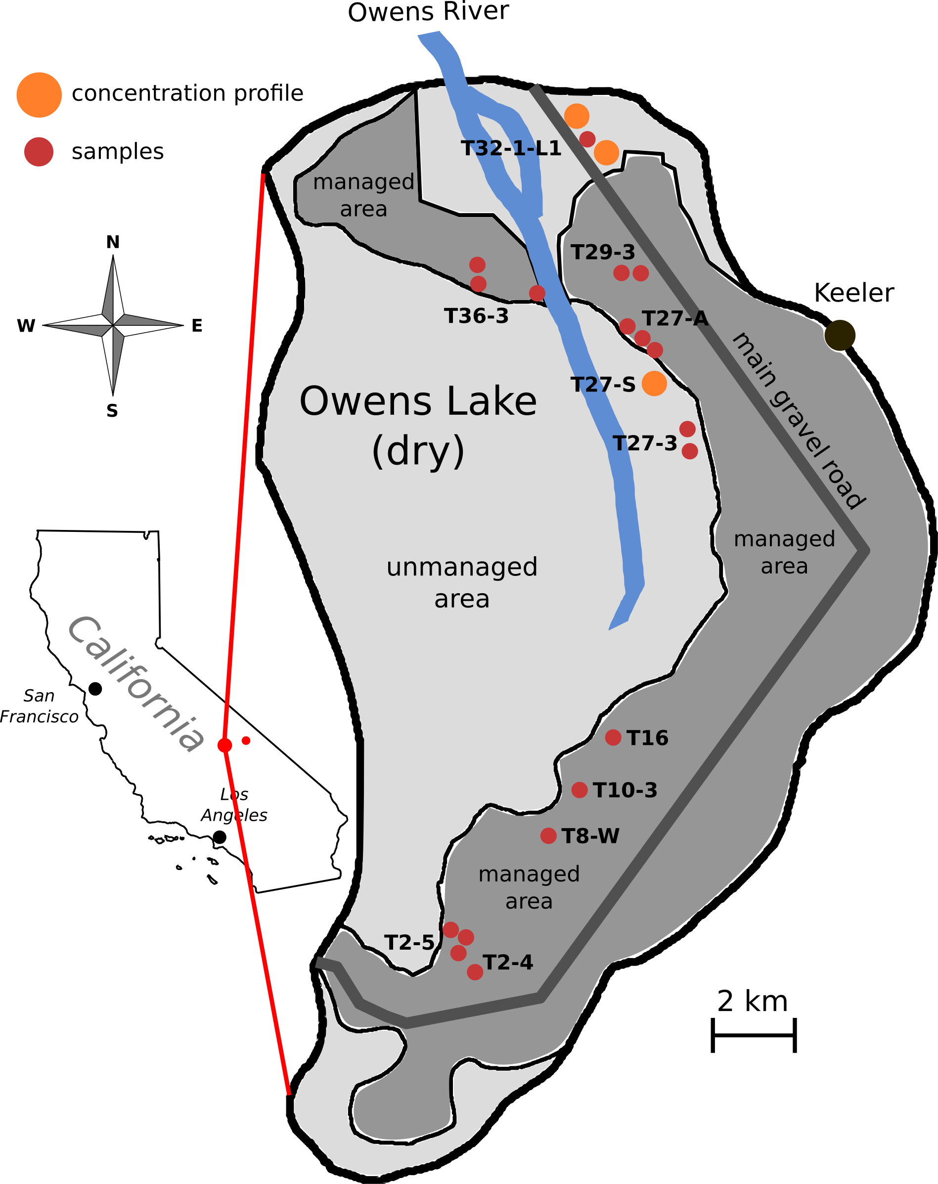
Figure 9 Schematic map of Owens Lake in central California, USA. Field sites are indicated as red (coring) and orange (trenching) dots.
Figure 10: Map of the field sites at Badwater Basin 
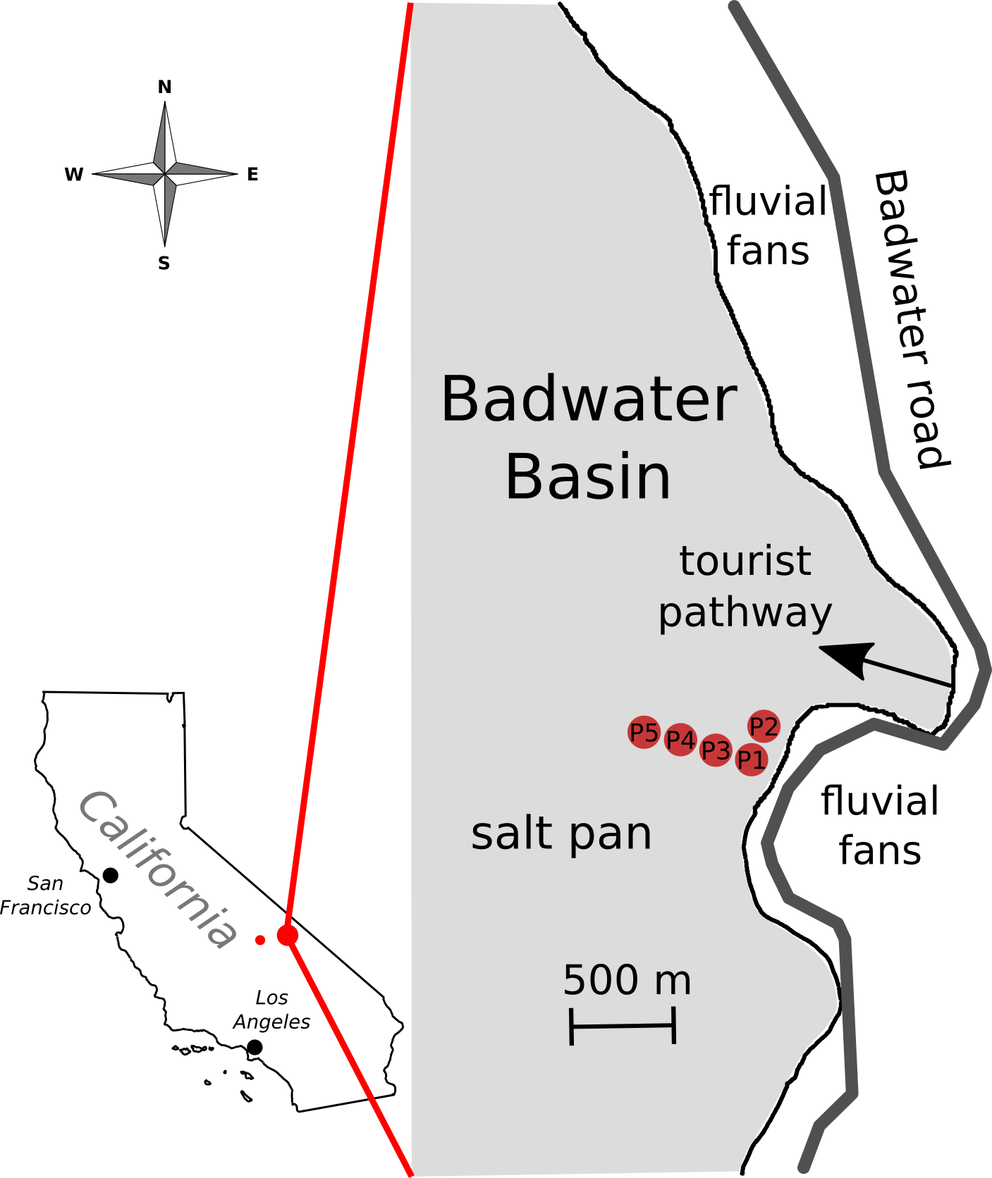
Figure 10 Schematic map of Badwater Basin in the Death Valley, central California, USA. Sampling sites (all coring) are indicated as red dots.
References 
[1] Gill, T. E. Eolian sediments generated by anthropogenic disturbance of playas: Humanimpacts on the geomorphic system and geomorphic impacts on the human system. Geomorphology 17, 207 – 228 (1996).
[2] Wadge, G., Archer, D. & Millington, A. Monitoring playa sedimentation using sequentialradar images. Terra Nova 6, 391–396 (1994).
[3] Lowenstein, T. K. & Hardie, L. A. Criteria for the recognition of salt-pan evaporites. Sedimentology 32, 627–644 (1985).
[4] Lokier, S. Development and evolution of subaerial halite crust morphologies in a coastalSabkha setting. J. Arid Environ. 79, 32 – 47 (2012).
[5] Nield, J. M.et al. Estimating aerodynamic roughness over complex surface terrain. J.Geophys. Res.: Atmos. 118, 12,948–12,961 (2013).
[6] Nield, J. M.et al. The dynamism of salt crust patterns on playas. Geology 43, 31 (2015).
[7] Prospero, J. M. Environmental characterization of global sources of atmospheric soildust identified with the NIMBUS 7 total ozone mapping spectrometer (TOMS) absorbing aerosol product. Rev. Geophys. 40 (2002).
[8] Fung, I. Y.et al. Iron supply and demand in the upper ocean. Global Biogeochem. Cy. 14, 281–295 (2000).
[9] Cahill, T. A., Gill, T. E., Reid, J. S., Gearhart, E. A. & Gillette, D. A. Saltating Particles,Playa Crusts and Dust Aerosols at Owens (dry) Lake, California. Earth Surf. Proc. Land. 21, 621–639 (1996).
[10] Gill, T. E., Gillette, D. A., Niemeyer, T. & Winn, R. T. Elemental geochemistry of wind-erodible playa sediments, Owens Lake, California. Nucl. Instrum. Meth. B 189, 209 – 213 (2002).
[11] Bryant, R. & Rainey, M. Investigation of flood inundation on playas within the Zone of Chotts, using a time-series of AVHRR. Remote Sens. Environ. 82, 360–375 (2002).
[12] Wooding, R. Rayleigh instability of a thermal boundary layer in flow through a porousmedium. J. Fluid Mech. 9, 183–192 (1960).
[13] Homsy, G. M. & Sherwood, A. E. Convective instabilities in porous media with throughflow. AIChE J. 22, 168–174 (1976).
[14] Wooding, R. A., Tyler, S. W., White, I. & Anderson, P. A. Convection in groundwaterbelow an evaporating Salt Lake: 2. Evolution of fingers or plumes. Water Resour. Res. 33, 1219–1228 (1997).
[15] Wooding, R. A. Variable-density saturated flow with modified Darcy’s law: The salt lakeproblem and circulation. Water Resour. Res. 43 (2007).
[16] Van Dam, R. L., Simmons, C. T., Hyndman, D. W. & Wood, W. W. Natural free convectionin porous media: First field documentation in groundwater. Geophysical Research Letters 36 (2009).
[17] Christiansen, F. W. Polygonal fracture and fold systems in the salt crust, Great Salt Lake Desert, Utah. Science 139, 607–609 (1963).
[18] Fryberger, S. G., Al-Sari, A. M. & Clisham, T. J. Eolian Dune, Interdune, Sand Sheet, and Siliciclastic Sabkha Sediments of an Offshore Prograding Sand Sea, Dhahran Area, SaudiArabia. AAPG Bulletin 67, 280–312 (1983).
[19] Krinsley, D. A geomorphological and paleoclimatological study of the playas of Iran. Part1. U.S. Geol. Survey CP 70-800 (1970).
[20] Dixon, J. C. Aridic Soils, Patterned Ground, and Desert Pavements, 101–122 (SpringerNetherlands, Dordrecht, 2009).
[21] Tucker, R. M. Giant polygons in the Triassic salt of Cheshire, England; a thermal contrac-tion model for their origin. J. of Sediment. Res. 51, 779 (1981).
[22] Deckker, P. D. Biological and sedimentary facies of australian salt lakes. Palaeogeogr. Palaeocl. 62, 237–270 (1988).
[23] Lachenbruch, A. H. Depth and spacing of tension cracks. Journal of Geophysical Research 66, 4273–4292 (1961).
[24] Groisman, A. & Kaplan, E. An experimental study of cracking induced by desiccation. Europhys. Lett. 25, 415–420 (1994).
[25] Shorlin, K. A., de Bruyn, J. R., Graham, M. & Morris, S. W. Development and geometryof isotropic and directional shrinkage-crack patterns. Phys. Rev. E 61, 6950–6957 (2000).
[26] Bowden, N., Brittain, S., Evans, A. G., Hutchinson, J. W. & Whitesides, G. M. Spontaneous formation of ordered structures in thin films of metals supported on an elastomericpolymer. Nature 393, 146–149 (1998).
[27] Li, B., Cao, Y.-P., Feng, X.-Q. & Gao, H. Mechanics of morphological instabilities andsurface wrinkling in soft materials: a review. Soft Matter 8, 5728 (2012).
[28] Gueler, C. & Thyne, G. D. Hydrologic and geologic factors controlling surface andgroundwater chemistry in Indian Wells - Owens Valley area, southeastern California, USA. J. Hydrol. 285, 177 – 198 (2004).
[29] Ryu, J., Zierenberg, R. A., Dahlgren, R. A. & Gao, S. Sulfur biogeochemistry and isotopic fractionation in shallow groundwater and sediments of Owens Dry Lake, California. Chem. Geol. 229, 257 – 272 (2006).
[30] Groeneveld, D. P. & Barz, D. D. Remote Monitoring of surfaces wetted for dust controlon the dry Owens lakebed, California. Open J. Mod. Hydro. 3, 241–252 (2013).
[31] Nicholas, L. & Andy, B. Influence of vegetation cover on sand transport by wind: fieldstudies at Owens Lake, California. Earth Surf. Proc. Land. 23, 69–82 (1997).
[32] Groeneveld, D., Huntington, J. & Barz, D. Floating brine crusts, reduction of evaporationand possible replacement of fresh water to control dust from Owens Lake bed, California. J. Hydrol. 392, 211 – 218 (2010).
[33] Slim, A. C. Solutal convection regimes in a two-dimensional porous medium. J. Fluid Mech. 741, 461–491 (2014).
[34] Lapwood, E. R. Convection of a fluid in a porous medium. Math. Proc. Cambridge 44, 508–521 (1948).
[35] Horton, C. W. & Rogers, F. T. Convection currents in a porous medium. J. Appl. Phys. 16, 367–370 (1945).
[36] Ernst, M. Numerical simulation of polygonal patterns in salt playa. Master’sthesis, University Gottingen (2017) URL.
[37] Sauter, J. Die Grössenbestimmung der in Gemischnebeln von Verbrennungskraftmaschinen vorhandenen Brennstoffteilchen. VDI-Forschungsheft 279 (1928).
[38] Tyler, S. et al. Estimation of groundwater evaporation and salt flux from Owens Lake,California, USA. J. Hydrol. 200, 110–135 (1997).
[39] Garcia, X., Akanji, L. T., Blunt, M. J., Matthai, S. K. & Latham, J. P. Numerical study ofthe effects of particle shape and polydispersity on permeability. Phys. Rev. E 80, 021304 (2009).
[40] Handford, C. R. Estimated ground-water discharge by evapotranspiration from Death Valley, California, 1997–2001. U.S. Geol. Survey 3 (2003).
[41] Brunner, P., Bauer, P., Eugster, M. & Kinzelbach, W. Using remote sensing to regionalize local precipitation recharge rates obtained from the Chloride Method. J. Hydrol. 294, 241–250 (2004).
[42] Nield, J. M., Neuman, C. M., O’Brien, P., Bryant, R. G. & Wiggs, G. F. Evaporativesodium salt crust development and its wind tunnel derived transport dynamics under vari-able climatic conditions. Aeolian Res. 23, 51–62 (2016).
[43] Slim, A. C., Bandi, M. M., Miller, J. C. & Mahadevan, L. Dissolution-driven convectionin a Hele-Shaw cell. Phys. Fluids 25, 024101 (2013).
[44] Thomas, C., Dehaeck, S. & Wit, A. D. Convective dissolution of CO$_2$ in water and saltsolutions. Int. J. Greenh. Gas Con. 72, 105–116 (2018).
[45] Juergens, N. The biological underpinnings of Namib desert fairy circles. Science 339, 1618–1621 (2013).
[46] Sletten, R. S. Resurfacing time of terrestrial surfaces by the formation and maturation ofpolygonal patterned ground. J. Geophys. Res. 108 (2003).
[47] Kessler, M. A. & Werner, B. T. Self-organization of sorted patterned ground. Science 299, 380–383 (2003).
[48] Goehring, L. Evolving fracture patterns: Columnar joints, mud cracks and polygonalterrain. Philos. T. R. Soc. A 371, 20120353–20120353 (2013).
[49] Shattuck, M. D., Behringer, R. P., Johnson, G. A. & Georgiadis, J. G. Convection and flowin porous media. Part 1: Visualization by magnetic resonance imaging. J. Fluid Mech. 332, 215–245 (1997).
[50] Hollet, K. J., Danskin, W. R., McCaffrey, W. F. & Waiti, C. L. Geology and water resources of Owens Valley California. U.S. Geol. Survey (1991).
[51] Hunt, C. B., Robinson, T., Bowles, W. & Washburn, A. Hydrologic basin, Death Valley,California. U.S. Geol. Survey (1966).
[52] Annunziata, O., Rard, J. A., Albright, J. G., Paduano, L. & Miller, D. G. Mutual diffusion coefficients and densities at 298.15 K of aqueous mixtures of NaCl and Na$_2$SO$_4$ for six different solute fractions at a total molarity of 1.500 mol·dm$^3$ and of aqueous Na$_2$SO$_4$. J. Chem. Eng. Data 45, 936–945 (2000).
[53] Boudreau, B. P. Diagenetic models and their implementation: Modelling transport and reactions in aquatic sediments (Springer, 2011).
[54] Boudreau, B. P. The diffusive tortuosity of fine-grained unlithified sediments. Geochim. Cosmochim. Ac. 60, 3139–3142 (1996).
[55] LADWP. Owens Lake habitat management plan (2010).
[56] Schindelin, J. et al. Fiji: an open-source platform for biological-image analysis. Nature Methods 9, 676–682 (2012).
[57] Riaz, A. & Meiburg, E. Three-dimensional miscible displacement simulations in homogeneous porous media with gravity override. J. Fluid Mech. 494, 95–117 (2003).
[58] Ruith, M. & Meiburg, E. Miscible rectilinear displacements with gravity override. Part 1: Homogeneous porous medium. J. Fluid Mech. 420, 225–257 (2000).
[59] Chen, C.-Y. Topics in miscible porous media flows (University of Southern California, 1998).
[60] Lele, S. K. Compact finite difference schemes with spectral-like resolution. J. Comput.Phys. 103, 16–42 (1992)
[61] Lasser, J. and Goehring, L. Grain size distributions of sand samples from Owens Lake and Badwater Basin in central California, collected in 2016 and 2018, DOI, (2020).