The Laplace Transform¶

This Jupyter notebook is part of a collection of notebooks in the bachelors module Signals and Systems, Communications Engineering, Universität Rostock. Please direct questions and suggestions to Sascha.Spors@uni-rostock.de.

Inverse Transform¶

So far only the (forward) Laplace transform has been introduced. The Laplace transform features also an inverse transform. The inverse Laplace transform maps a complex-valued Laplace transform $X(s) \in \mathbb{C}$ with complex-valued independent variable $s \in \mathbb{C}$ into the complex-valued signal $x(t) \in \mathbb{C}$ with real-valued independent variable $t \in \mathbb{R}$. It can be shown that the inverse Laplace transform $x(t) = \mathcal{L}^{-1} \{ X(s) \}$ is uniquely determined for most practically relevant signals. This section discusses two different techniques for the computation of the inverse Laplace transform.

Integral Formula¶

Using results from complex analysis, the inverse Laplace transform is given by the following complex line integral

\begin{equation} x(t) = \frac{1}{2 \pi j} \int_{\sigma - j \infty}^{\sigma + j \infty} X(s) \, e^{s t} \; ds \end{equation}

where $X(s) = \mathcal{L} \{ x(t) \}$ is assumed to be analytic in its simply connected region of convergence (ROC). The notation $\sigma \mp j \infty$ for the lower/upper integration limit denotes an arbitrary integration path which lies in the ROC and ranges from $\Im \{s\} = - \infty$ to $\Im \{s\} = + \infty$. The integration path can be chosen parallel to the imaginary axis but also all other paths in the ROC are possible. This results from Cauchy's integral theorem. Two equivalent paths are shown in the following illustration

Possible integration paths for the inverse Laplace transform

where the blue line indicates the integration path and the gray area the ROC.

Rational Laplace Transforms¶

Computing the inverse Laplace transform by above integral formula can be challenging. The Cauchy residue theorem provides a practically tractable solution for Laplace transforms $X(s) = \mathcal{L} \{ x(t) \}$ which are given as rational functions. It states that the value of a line integral of an holomorphic function over a closed contour is given by summing up its residues. The residue is the value of the line integral for a path enclosing a singularity. Consequently, the inverse Laplace transform of a rational Laplace transform can be computed by summing up the individual contributions from its poles. This procedure is detailed in the following.

Basic Procedure¶

A rational Laplace transform $X(s)$ can be written in terms of its numerator and denominator polynomial

\begin{equation} X(s) = \frac{\sum_{m=0}^{M} \beta_m s^m}{\sum_{n=0}^{N} \alpha_n s^n} \end{equation}

where $M$, $N$ denote the order of the numerator and denominator polynomial and $\beta_m$, $\alpha_n$ their coefficients, respectively. It is assumed that $\alpha_N \neq 0$ and that $M \leq N$. If $M > N$, $X(s)$ can be decomposed by polynomial division into a sum of powers of $s$ and a rational function fulfilling $M \leq N$.

Now a partial fraction decomposition of $X(s)$ is performed resulting in

\begin{equation} X(s) = A_0 + \sum_{\mu = 1}^{L} \sum_{\nu = 1}^{R_\mu} \frac{A_{\mu \nu}}{(s - s_{\infty \mu})^\nu} \end{equation}

where $s_{\infty \mu}$ denotes the $\mu$-th unique pole of $X(s)$, $R_\mu$ its degree and $L$ the total number of different poles $\mu = 1 \dots L$. Using the known Laplace transforms (cf. example for the modulation theorem or table of selected transforms)

\begin{equation} \mathcal{L} \{ t^n e^{-s_0 t} \epsilon(t) \} = \frac{n!}{(s + s_0)^{n+1}} \qquad \text{for } \Re \{ s \} > \Re \{ - s_0 \} \end{equation}

and $\mathcal{L} \{ \delta(t) \} = 1$, together with the linearity of the Laplace transform yields a generic result for the inverse Laplace transform $x(t) = \mathcal{L}^{-1} \{ X(s) \}$ of a right-sided signal

\begin{equation} x(t) = A_0 \cdot \delta(t) + \epsilon(t) \sum_{\mu = 1}^{L} e^{s_{\infty \mu} t} \sum_{\nu = 1}^{R_\mu} \frac{A_{\mu \nu} \, t^{\mu - 1}}{(\nu -1)!} \end{equation}

It remains to compute the coefficients $A_0$ and $A_{\mu \nu}$ of the partial fraction decomposition. The constant coefficient $A_0$ is given as

\begin{equation} A_0 = \lim_{s \to \infty} X(s) \end{equation}

For a pole $s_{\infty \mu}$ with degree $R_\mu = 1$, the coefficient $A_{\mu 1}$ reads

\begin{equation} A_{\mu 1} = \lim_{s \to s_{\infty \mu}} \left( X(s) \cdot (s - s_{\infty \mu}) \right) \end{equation}

For a pole $s_{\infty \mu}$ of degree $R_\mu > 1$, the coefficients $A_{\mu \nu}$ are given as

\begin{equation} A_{\mu \nu} = \frac{1}{(R_\mu - \nu)!} \lim_{s \to s_{\infty \mu}} \frac{d^{R_\mu - \nu}}{d s^{R_\mu - \nu}} \left( X(s) \cdot (s - s_{\infty \mu})^{R_\mu} \right) \end{equation}

Example - Inverse transform of a rational Laplace transform¶

The inverse transform $x(t) = \mathcal{L}^{-1} \{ X(s) \}$ of

\begin{equation} X(s) = \frac{1}{(s+1) (s+2)^2} \qquad \text{for } \Re \{s \} > -1 \end{equation}

is computed using the procedure outline above. First the function $X(s)$ is defined in SymPy

In [1]:

import sympy as sym
%matplotlib inline
sym.init_printing()

s = sym.symbols('s', complex=True)
t = sym.symbols('t', real=True)

X = 1/((s+1)*(s+2)**2)
X

Out[1]:

$$\frac{1}{\left(s + 1\right) \left(s + 2\right)^{2}}$$

Since $X(s)$ has two real-values poles, $x_{\infty 1} = -1$ with degree $R_1 = 1$ and $x_{\infty 2} = -2$ with degree $R_2 = 2$, the following partial fraction decomposition is chosen as ansatz in accordance with above given formula

In [2]:

A0, A11, A21, A22 = sym.symbols('A_0 A_{11} A_{21} A_{22}', real=True)
Xp = A0 + A11/(s+1) + A21/(s+2) + A22/(s+2)**2
Xp

Out[2]:

$$A_{0} + \frac{A_{11}}{s + 1} + \frac{A_{21}}{s + 2} + \frac{A_{22}}{\left(s + 2\right)^{2}}$$

The four real-valued constants $A_0$, $A_{11}$, $A_{21}$ and $A_{22}$ of the partial fraction decomposition will be determined later. First a look is taken at the inverse Laplace transforms of the individual summands composed from the constant and the individual poles. For the constant we get

In [3]:

x0 = sym.inverse_laplace_transform(Xp.args[0], s, t)
x0

Out[3]:

$$A_{0} \delta\left(t\right)$$

For the first pole $s_{\infty 1}$ with degree zero we get

In [4]:

x1 = sym.inverse_laplace_transform(Xp.args[1], s, t)
x1

Out[4]:

$$A_{11} e^{- t} \theta\left(t\right)$$

For the second pole $s_{\infty 2}$ with degree two we get two contributions

In [5]:

x2 = sym.inverse_laplace_transform(Xp.args[2], s, t)
x2

Out[5]:

$$A_{21} e^{- 2 t} \theta\left(t\right)$$

In [6]:

x3 = sym.inverse_laplace_transform(Xp.args[3], s, t)
x3

Out[6]:

$$A_{22} t e^{- 2 t} \theta\left(t\right)$$

The inverse Laplace transform of $X(s)$ is now composed from the superposition of the four individual parts

In [7]:

x = x0 + x1 + x2 + x3
x

Out[7]:

$$A_{0} \delta\left(t\right) + A_{11} e^{- t} \theta\left(t\right) + A_{21} e^{- 2 t} \theta\left(t\right) + A_{22} t e^{- 2 t} \theta\left(t\right)$$

For the final solution the four coefficients are determined using the given limit formulas for the coefficients of a partial fraction decomposition

In [8]:

coeffs = {A0 : sym.limit(X, s, sym.oo)}
coeffs.update({A11 : sym.limit(X*(s+1), s, -1)})
coeffs.update({A21 : sym.limit(sym.diff(X*(s+2)**2, s), s, -2)})
coeffs.update({A22 : sym.limit(X*(s+2)**2, s, -2)})
coeffs

Out[8]:

$$\left \{ A_{0} : 0, \quad A_{11} : 1, \quad A_{21} : -1, \quad A_{22} : -1\right \}$$

Substitution into the inverse Laplace transform yields the final solution $x(t) = \mathcal{L}^{-1}\{ X(s) \}$

In [9]:

x = x.subs(coeffs)
x

Out[9]:

$$- t e^{- 2 t} \theta\left(t\right) + e^{- t} \theta\left(t\right) - e^{- 2 t} \theta\left(t\right)$$

The solution is plotted for illustration

In [10]:

sym.plot(x, (t, -1, 10), ylabel=r'$x(t)$')

Out[10]:

<sympy.plotting.plot.Plot at 0x11e8f46a0>

Exercise

Derive the inverse Laplace transform of $X(s)$ by manual calculation.

Classification of Poles¶

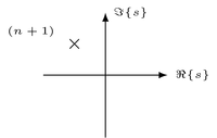
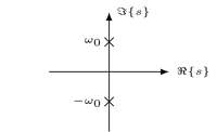
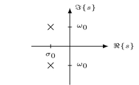
Above procedure allows to compute the inverse Laplace transform $x(t) = \mathcal{L}^{-1} \{ X(s) \}$ of a rational Laplace transform $X(s)$ in a systematic way. It is well suited for an algorithmic realization. However, for manual calculus it may be more efficient to classify the poles with respect to their location in the $s$-plane and their symmetries. The classification can then be used to formulate a modified partial fraction decomposition which limits the need for later algebraic simplification of the inverse Laplace transform. Three classes of poles are typically considered

Type	$X(s)$	$x(t) = \mathcal{L}^{-1} \{ X(s) \} \qquad \qquad$
Single complex pole	$\frac{n!}{(s + s_0)^{n+1}}$	$t^n e^{-s_0 t} \epsilon(t)$
Conjugated imaginary poles	$\frac{A s + B}{s^2 + \omega_0^2}$	$\begin{cases} \sin(\omega_0 t) \epsilon(t) \\ \cos(\omega_0 t) \epsilon(t) \end{cases}$
Conjugated complex poles	$\frac{A s + B}{(s + \sigma_0)^2 + \omega_0^2}$	$\begin{cases} e^{-\sigma_0 t} \sin(\omega_0 t) \epsilon(t) \\ e^{-\sigma_0 t} \cos(\omega_0 t) \epsilon(t) \end{cases}$

where $s_0 \in \mathbb{C}$ and $\omega_0, \sigma_0 \in \mathbb{R}$. The expansion coefficients $A, B \in \mathbb{R}$ can be derived by comparison of coefficients. Whether $x(t)$ contains a sine or cosine depends on the coefficient $A$. If $A \neq 0$ then $x(t)$ contains a cosine (cf. table of selected transforms).

Example - Inverse transform of a rational Laplace transform with symmetric poles¶

The inverse transform $x(t) = \mathcal{L}^{-1} \{ X(s) \}$ of

\begin{equation} X(s) = \frac{2 s^2 + 14 s + 124}{s^3 + 8 s^2 + 46 s + 68} \qquad \text{for } \Re \{s \} > -2 \end{equation}

is computed. First the function $X(s)$ is defined in SymPy

In [11]:

X = (2*s**2 + 14*s + 124)/(s**3 + 8 * s**2 + 46*s + 68)
X

Out[11]:

$$\frac{2 s^{2} + 14 s + 124}{s^{3} + 8 s^{2} + 46 s + 68}$$

The poles of $X(s)$ are derived by computing the roots of the denominator polynomial

In [12]:

poles = sym.roots(sym.denom(X))
poles

Out[12]:

$$\left \{ -2 : 1, \quad -3 - 5 i : 1, \quad -3 + 5 i : 1\right \}$$

The result is a real-valued pole and a conjugate complex pair of poles. According to above introduced classification of poles, the following ansatz is chosen for the partial fraction decomposition of the Laplace transform

\begin{equation} X_p(s) = \frac{A}{s + 2} + \frac{B s + C}{s^2 + 6s + 34} \end{equation}

The coefficients $A, B, C \in \mathbb{R}$ are derived by equating coefficients with $X(s)$

In [13]:

A, B, C = sym.symbols('A B C', real=True)

Xp = A / (s+2) + (B*s + C)/(s**2 + 6*s + 34)
coeffs = sym.solve(sym.Eq(X, Xp), (A, B, C))
coeffs

Out[13]:

$$\left \{ A : 4, \quad B : -2, \quad C : -6\right \}$$

Introducing the coefficients into $X_p(s)$ yields

In [14]:

Xp = Xp.subs(coeffs)
Xp

Out[14]:

$$\frac{- 2 s - 6}{s^{2} + 6 s + 34} + \frac{4}{s + 2}$$

The first fraction belongs to the complex conjugate poles. Applying completion of the square to the denominator, its inverse can be identified in the table of Laplace transforms as exponentially decaying cosine signal. Performing the inverse Laplace transform with SymPy yields

In [15]:

x1 = sym.inverse_laplace_transform(Xp.args[1], s, t)
x1

Out[15]:

$$- 2 e^{- 3 t} \cos{\left (5 t \right )} \theta\left(t\right)$$

The second fraction belongs to a real-valued pole of first degree. Its inverse Laplace transform can be looked-up directly in the table of Laplace transforms as exponentially decaying signal. Performing the inverse Laplace transform again with SymPy yields

In [16]:

x2 = sym.inverse_laplace_transform(Xp.args[0], s, t)
x2

Out[16]:

$$4 e^{- 2 t} \theta\left(t\right)$$

The inverse Laplace transform of $X(s)$ is given by summing up these two parts

In [17]:

x = x1 + x2
x

Out[17]:

$$4 e^{- 2 t} \theta\left(t\right) - 2 e^{- 3 t} \cos{\left (5 t \right )} \theta\left(t\right)$$

The resulting signal is plotted for illustration

In [18]:

sym.plot(x, (t, -0.1, 4), xlabel='$t$', ylabel='$x(t)$');

The same result can be derived directly from $X(s)$ by using the inverse Laplace transform of SymPy

In [19]:

sym.inverse_laplace_transform(X, s, t).simplify()

Out[19]:

$$2 \left(2 e^{t} - \cos{\left (5 t \right )}\right) e^{- 3 t} \theta\left(t\right)$$

Exercise

Derive the inverse Laplace transform of $X(s)$ by manual calculation.

Copyright

The notebooks are provided as Open Educational Resource. Feel free to use the notebooks for your own educational purposes. The text is licensed under Creative Commons Attribution 4.0, the code of the IPython examples under the MIT license. Please attribute the work as follows: Lecture Notes on Signals and Systems by Sascha Spors.