Stereo Model and Camera Calibration¶

Kevin J. Walchko, Phd

20 Nov 2018

Stereo Vision is utilizing 2 (or more) pinhole cameras. We typically use a similar model to explaine geometry, but since we have more than one camera, we can get depth (z-direction) information.

References¶

• [1] camera.pdf
• [2] [Multiple View Geometry in Computer Vision

Second Edition](http://www.robots.ox.ac.uk/~vgg/hzbook/hzbook2/HZepipolar.pdf)

• [3] CSE486, lecture 19
• wikipedia: Fundamental Matrix (F)
• wikipedia: Essential Matrix (E)
• github: StereoVision
• github: steroid
• github: OpenCV Python Tutorials
• gist: Adhoc AR Tracker for Planar Scenes
• github.io: Stereo Calibration Demo
• ROS: Choosing Good Stereo Parameters
• sourishghosh: Stereo Calibration using C++
• sourishghosh: Calculating the Fundamental Matrix
• kushalvyas: Demystifying Geometrix Camera Calibration
• GeorgiaTech: CS4476: Camera Calibration and Fundamental Matrix
• CalTech: Matlab Camera Calibration Toolbox

Calibrating Stereo Cameras¶

We will look a calibrating a stereo camera using the standard chessboard pattern.

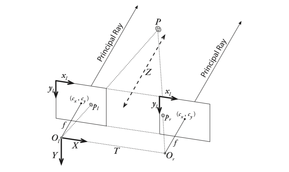
We need to estimate some camera parameters, both internal and external. Basic process:

1. For a series of images, use cv2.findMarkers() to find your calibration target's pattern (objpts) in the image (imgpts) for each gray scale image
   • objpts are how the features exist in the 3D world
   • imgpts are how the same features appear in the 2D image
2. You can use cv2.cornerSubPix() to refine your results
   • Sometimes this degrades the results instead of improves them
3. Use cv2.calibrateCamera() to get the left/right camera intrinsic parameters
   • You will run this twice, once on each camera
   • The key results are the camera matrix (K) and the distortion coefficients (d) for each
4. Use cv2.stereoCalibrate() to get the system extrinsic parameters
   • Rotation (R): How the right camera is rotated relative to the left camera
   • Translation (T): The distance the right camera is from the left camera (units will be meters, centimeters, milimeters, etc)
   • Essential Matrix (E): contains the information about translation and rotation between the 2 cameras in global coordinates.
   • Fundamental Matrix (F): contains the same information as E, but also contains intrinsics of both cameras so that we can relate the two cameras in pixel coordinates.

Now we have a set of parameters:

• Camera matrix: K1, K2
• Projection matrix:
  • Left: $P1 = K1 [I|0]$
  • Right: $P2 = K2 [R|T]$
• Fundamental matrix[2]: $F = K2^{-T}RK1^T [K1 R^T t]_x$ where $[]_x$ is the skew matrix
  • Uses image coordinates both the intrinsics and extrinsics
  • Derivation found in 2 Table 9.1, bottom
• Essential matrix
  • $E = R [R^T t]_x$
  • Can also be found from: $E = K2^T F K1$ [2, eqn 9.12]
  • Uses camera coordinate and only needs the extrinsics

Epipolar Lines¶

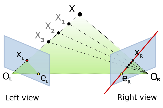
Stereo matching generally utilizes searching across epipolar lines for features that match. This helps to greatly reduce the search space and speed things up. The essential and fundamental matricies encode the epipolar geometery between two views of the same objects. An epipolar line:

$$ au+bv+c=0 \\ p = \begin{bmatrix} u & v & 1 \end{bmatrix}^T \\ l = \begin{bmatrix} a & b & c \end{bmatrix}^T \\ p^Tl = l^Tp = 0 $$

It turns out we can use these equations for epipolar lines and subtitute in $E$ or $F$.

$$ p^T_1 l_1 = p^T_1 E p_2 = 0 $$

where $p_1$ a point in the left camera and $p_2$ is a point in the right camera.

Like F, E carries knowledge of the stereo setup, but it exists in normalized space, not pixel space.

$$ \begin{eqnarray} \hat x' = R(\hat x -T) \\ E = R[t]_x \\ [t]_x = \begin{bmatrix} 0 & -T_z & T_y \\ T_z & 0 & -T_x \\ -T_y & T_x & 0 \end{bmatrix} \end{eqnarray} $$

Given image points in both cameras (with noise), the E can be estimated using a total least squares approach. This approach is commonly referred to as the eight-point-algorithm

See CSE486 [3] for examples of finding $F$ and calculating epipolar lines.

Rectifying Images¶

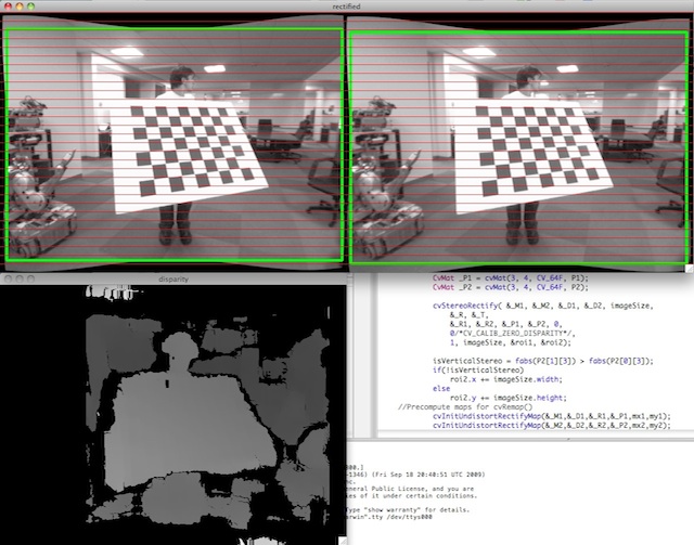
During camera manufacturing, small mechanical misalignments are produced which can effect stereo performance. To fix the image and make straight lines (think epipolar lines) straight again:

• cv2.stereoRectify() to produce necessary matricies
• Create distortion maps using cv2.initUndistortRectifyMap() for the left/right camera
• Undistort an image using cv2.remap() and the products from the above functions. The good thing, though, is the first 2 function can be called once so you have everything. Then, during run-time, you can just use cv2.remap()

Calculating Disparity Maps¶

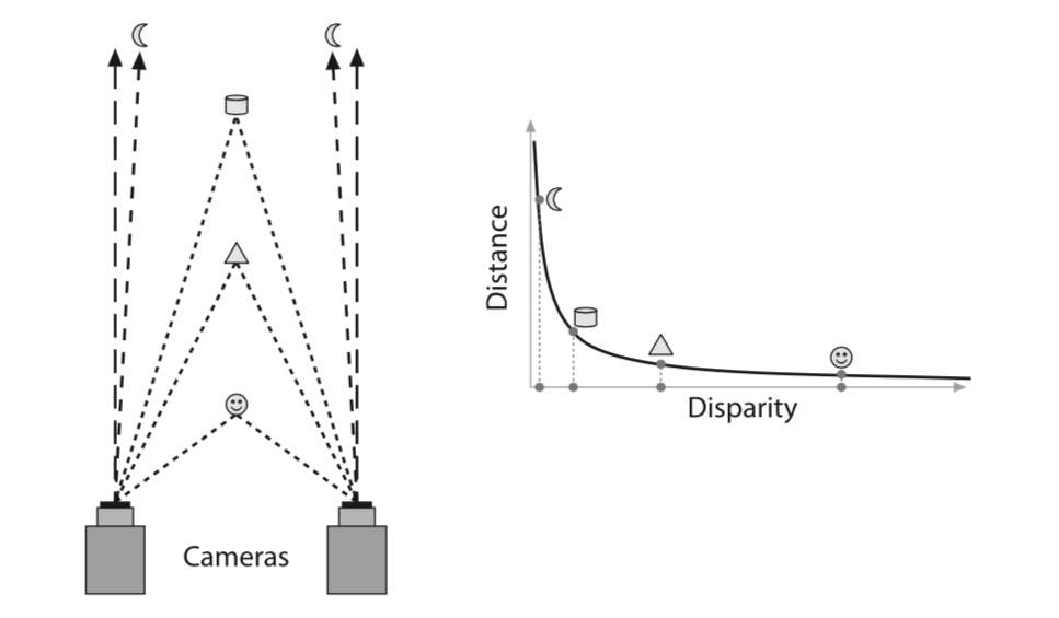
Objects closer to the stereo cameras will have larger disparity, meaning they will be found in different places in the two images. Conversly, objects farther way will have smaller disparity and will be found roughly in the same row/column of both images.

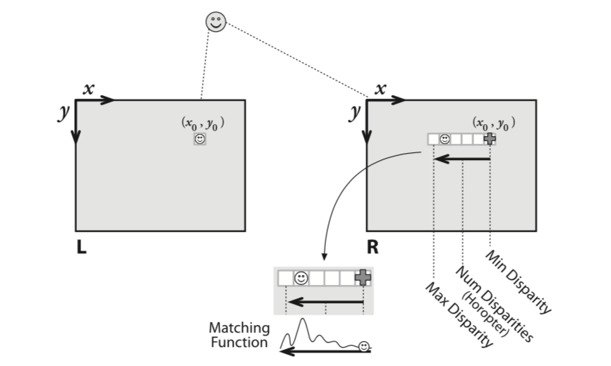
Stereo models like cv2.StereoSGBM or cv2.StereoBM can be used to find corresponding points in the image pair (left and right) and calculate the disparity between them (number of pixels). Instead of matching individual pixels, the stereo models tend to match blocks of pixels.

Basic process¶

1. Rectify images to ensure epipolar constraint
2. Find features in both individual images
3. Match each feature in the left image to a feature in the right image
   • You don't want to search the entire image, takes too much time
   • Reduce search by looking along epipolar lines
4. (see image above) Given feature at p(x,y) in the left image
   • Start at the minimum disparity (matcher parameter) and move left along epipolar line until you:
     • Find a match and record the distance ($p_{right} - p_{left}$)
       • Sometimes the syntax $x - x'$ is used for disparity
     • Or hit the maximum disparity (matcher parameter) and give up for that feature
       • NaN means the feature couldn't be matched
     • Iterate across all features
5. Filter out bad matches that result in error (i.e., $disp \le 0$)
   • Valid numbers range from disparity.min() to (disparity.min()+numDisparities)

Block Matching (BM)¶

OpenCV 3.4 docs: ref

The class computing stereo correspondence using the block matching algorithm, introduced and contributed to OpenCV by K. Konolige. Stereo algorithms tend not to match points (which is what the math above leads you to believe) but rather they match square blocks of pixels (e.g., 5x5, 7x7).

Params¶

• numDisparities: the disparity search range. For each pixel algorithm will find the best disparity from 0 (default minimum disparity) to numDisparities. The search range can then be shifted by changing the minimum disparity.
• blockSize: the linear size of the blocks compared by the algorithm. The size should be odd (as the block is centered at the current pixel). Larger block size implies smoother, though less accurate disparity map. Smaller block size gives more detailed disparity map, but there is higher chance for algorithm to find a wrong correspondence.

Semi Global Block Matching (SGBM)¶

OpenCV 3.4 docs: ref

The class implements the modified H. Hirschmuller algorithm that differs from the original one as follows:

• By default, the algorithm is single-pass, which means that you consider only 5 directions instead of 8. Set mode=StereoSGBM::MODE_HH in StereoSGBM_create to run the full variant of the algorithm but beware that it may consume a lot of memory.
• The algorithm matches blocks, not individual pixels. Though, setting blockSize=1 reduces the blocks to single pixels.
• Mutual information cost function is not implemented. Instead, a simpler Birchfield-Tomasi sub-pixel metric from is used. Though, the color images are supported as well.
• Some pre- and post- processing steps from K. Konolige algorithm StereoBM are included, for example: pre-filtering (StereoBM::PREFILTER_XSOBEL type) and post-filtering (uniqueness check, quadratic interpolation and speckle filtering).

Params¶

• minDisparity: Minimum possible disparity value. Normally, it is zero but sometimes rectification algorithms can shift images, so this parameter needs to be adjusted accordingly.
• numDisparities: Maximum disparity minus minimum disparity. The value is always greater than zero. In the current implementation, this parameter must be divisible by 16.
• blockSize: Matched block size. It must be an odd number >=1 . Normally, it should be somewhere in the 3..11 range.
• P1: The first parameter controlling the disparity smoothness. See below.
• P2: The second parameter controlling the disparity smoothness. The larger the values are, the smoother the disparity is. P1 is the penalty on the disparity change by plus or minus 1 between neighbor pixels. P2 is the penalty on the disparity change by more than 1 between neighbor pixels. The algorithm requires P2 > P1 . See stereo_match.cpp sample where some reasonably good P1 and P2 values are shown, like:
  • P1: $8 \cdot numberImageChannels \cdot SADWindowSize \cdot SADWindowSize$
  • P2: $32 \cdot numberImageChannels \cdot SADWindowSize \cdot SADWindowSize$
  • where SAD is sum of absolute difference
• disp12MaxDiff: Maximum allowed difference (in integer pixel units) in the left-right disparity check. Set it to a non-positive value to disable the check.
• preFilterCap: Truncation value for the prefiltered image pixels. The algorithm first computes x-derivative at each pixel and clips its value by [-preFilterCap, preFilterCap] interval. The result values are passed to the Birchfield-Tomasi pixel cost function.
• uniquenessRatio: Margin in percentage by which the best (minimum) computed cost function value should "win" the second best value to consider the found match correct. Normally, a value within the 5-15 range is good enough.
• speckleWindowSize: Maximum size of smooth disparity regions to consider their noise speckles and invalidate. Set it to 0 to disable speckle filtering. Otherwise, set it somewhere in the 50-200 range.
• speckleRange: Maximum disparity variation within each connected component. If you do speckle filtering, set the parameter to a positive value, it will be implicitly multiplied by 16. Normally, 1 or 2 is good enough.
• mode: Set it to StereoSGBM::MODE_HH to run the full-scale two-pass dynamic programming algorithm. It will consume O(W*H*numDisparities) bytes, which is large for 640x480 stereo and huge for HD-size pictures. By default, it is set to False.

How to Get Good Disparity Map¶

1. Scene needs enough detectable and distinguishable features between image pairs
2. Need features appropriate for baseline
   • Features too close won't be seen in both images
   • Features too far will be reported as same pixel

Calibration¶

Rectification with cv2.stereoRectify()¶