Far-Field Profile of a Cavity
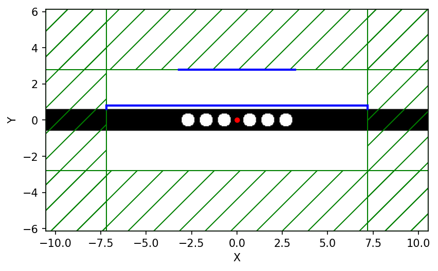
For this demonstration, we will compute the far-field spectra of a resonant cavity mode in a holey waveguide; a structure we had explored in Tutorial/Resonant Modes and Transmission in a Waveguide Cavity. The structure is shown in the left image below.
To set this up, we simply remove the last portion of examples/holey-wvg-cavity.py, beginning right after the line:
sim.symmetries.append(mp.Mirror(mp.Y, phase=-1))
sim.symmetries.append(mp.Mirror(mp.X, phase=-1))
and insert the following lines:
d1 = 0.2

sim = mp.Simulation(cell_size=cell,
                    geometry=geometry,
                    sources=[sources],
                    symmetries=symmetries,
                    boundary_layers=[pml_layers],
                    resolution=resolution)

nearfield = sim.add_near2far(
    fcen, 0, 1,
    mp.Near2FarRegion(mp.Vector3(0, 0.5 * w + d1), size=mp.Vector3(2 * dpml - sx)),
    mp.Near2FarRegion(mp.Vector3(-0.5 * sx + dpml, 0.5 * w + 0.5 * d1), size=mp.Vector3(0, d1), weight=-1.0),
    mp.Near2FarRegion(mp.Vector3(0.5 * sx - dpml, 0.5 * w + 0.5 * d1), size=mp.Vector3(0, d1))
)
We are creating a "near" bounding surface, consisting of three separate regions surrounding the cavity, that captures all outgoing waves in the top-half of the cell. Note that the x-normal surface on the left has a weight of -1 corresponding to the direction of the outward normal vector relative to the x direction so that the far-field spectra is correctly computed from the outgoing fields, similar to other DFT-field derived quantities such as flux and force. The parameter d1 is the distance between the edge of the waveguide and the bounding surface, as shown in the schematic above, and we will demonstrate that changing this parameter does not change the far-field spectra which we compute at a single frequency corresponding to the cavity mode.
We then time step the fields until they have sufficiently decayed away as the cell is surrounded by PMLs, and output the far-field spectra over a rectangular area that lies outside of the cell:
sim.run(until_after_sources=mp.stop_when_fields_decayed(50, mp.Hz, mp.Vector3(0.12, -0.37), 1e-8))

d2 = 20
h = 4

sim.output_farfields(nearfield, "spectra-{}-{}-{}".format(d1, d2, h), resolution,
                     mp.Volume(mp.Vector3(0, (0.5 * w) + d2 + (0.5 * h)), size=mp.Vector3(sx - 2 * dpml, h)))
The first item to note is that the far-field region is located outside of the cell, although in principle it can be located anywhere. The second is that the far-field spectra can be interpolated onto a spatial grid that has any given resolution but in this example we used the same resolution as the simulation. Note that the simulation itself used purely real fields but the output, given its analytical nature, contains complex fields. Finally, given that the far-field spectra is derived from the Fourier-transformed fields which includes an arbitrary constant factor, we should expect an overall scale and phase difference in the results obtained using the near-to-far-field feature with those from a corresponding simulation involving the full computational volume. The key point is that the results will be qualitatively but not quantitatively identical. The data will be written out to an HDF5 file having a filename prefix with the values of the three main parameters. This includes the far-field spectra for all six field components, including real and imaginary parts.
We run the above modified control file and in post-processing create an image of the real and imaginary parts of H$_z$ over the far-field region which is shown in insets (a) above. For comparison, we compute the steady-state fields using a larger cell that contains within it the far-field region. This involves a continuous source and complex fields. Results are shown in inset (b) of the figure above. The difference in the relative phases among any two points within each of the two field spectra is zero, which can be confirmed numerically. Also, as would be expected, it can be shown that increasing d1 does not change the far-field spectra as long as the results are sufficiently converged. This indicates that discretization effects are irrelevant.
In general, it is tricky to interpret the overall scale and phase of the far fields, because it is related to the scaling of the Fourier transforms of the near fields. It is simplest to use the near2far feature in situations where the overall scaling is irrelevant, e.g. when you are computing a ratio of fields in two simulations, or a fraction of the far field in some region, etcetera.
import meep as mp
import numpy as np
import matplotlib.pyplot as plt

resolution = 20  # pixels/μm

eps = 13  # dielectric constant of waveguide
w = 1.2  # width of waveguide
r = 0.36  # radius of holes
d = 1.4  # defect spacing (ordinary spacing = 1)
N = 3  # number of holes on either side of defect

sy = 6  # size of cell in y direction (perpendicular to wvg.)
pad = 2  # padding between last hole and PML edge
dpml = 1  # PML thickness
sx = 2 * (pad + dpml + N) + d - 1  # size of cell in x direction

cell = mp.Vector3(sx, sy, 0)
pml_layers = mp.PML(dpml)

geometry = [
    mp.Block(
        center=mp.Vector3(),
        size=mp.Vector3(mp.inf, w, mp.inf),
        material=mp.Medium(epsilon=eps),
    )
]

for i in range(N):
    geometry.append(mp.Cylinder(r, center=mp.Vector3(0.5 * d + i)))
    geometry.append(mp.Cylinder(r, center=mp.Vector3(-0.5 * d - i)))

fcen = 0.25  # pulse center frequency
df = 0.2  # pulse width (in frequency)

sources = mp.Source(
    src=mp.GaussianSource(fcen, fwidth=df), component=mp.Hz, center=mp.Vector3()
)

symmetries = [mp.Mirror(mp.X, phase=-1), mp.Mirror(mp.Y, phase=-1)]

sim = mp.Simulation(
    cell_size=cell,
    geometry=geometry,
    sources=[sources],
    symmetries=symmetries,
    boundary_layers=[pml_layers],
    resolution=resolution,
)

d1 = 0.2

nearfield = sim.add_near2far(
    fcen,
    0,
    1,
    mp.Near2FarRegion(mp.Vector3(y=0.5 * w + d1), size=mp.Vector3(sx - 2 * dpml)),
    mp.Near2FarRegion(
        mp.Vector3(-0.5 * sx + dpml, 0.5 * w + 0.5 * d1),
        size=mp.Vector3(y=d1),
        weight=-1.0,
    ),
    mp.Near2FarRegion(
        mp.Vector3(0.5 * sx - dpml, 0.5 * w + 0.5 * d1), size=mp.Vector3(y=d1)
    ),
)

sim.run(
    until_after_sources=mp.stop_when_fields_decayed(
        50, mp.Hz, mp.Vector3(0.12, -0.37), 1e-8
    )
)
-----------
Initializing structure...
field decay(t = 50.025000000000006): 61.714437239634854 / 61.714437239634854 = 1.0
field decay(t = 100.05000000000001): 47.39669513065221 / 61.714437239634854 = 0.7680001187827836
field decay(t = 150.07500000000002): 38.753487484300784 / 61.714437239634854 = 0.6279484868965497
field decay(t = 200.10000000000002): 31.933885594488228 / 61.714437239634854 = 0.517445949810579
field decay(t = 250.125): 26.076764607720868 / 61.714437239634854 = 0.42253912980630065
field decay(t = 300.15000000000003): 21.47655605320123 / 61.714437239634854 = 0.34799889643015885
field decay(t = 350.175): 17.53631126728562 / 61.714437239634854 = 0.2841524941593938
field decay(t = 400.20000000000005): 14.443563832839763 / 61.714437239634854 = 0.2340386541443446
field decay(t = 450.225): 11.896373926780527 / 61.714437239634854 = 0.19276484496791815
field decay(t = 500.25): 9.718573927428102 / 61.714437239634854 = 0.15747650569495178
field decay(t = 550.275): 8.004609807436562 / 61.714437239634854 = 0.12970400712486385
field decay(t = 600.3000000000001): 6.537545155581314 / 61.714437239634854 = 0.10593218455831122
field decay(t = 650.325): 5.384562849608928 / 61.714437239634854 = 0.08724964676743095
field decay(t = 700.35): 4.396534866374258 / 61.714437239634854 = 0.071239973384229
field decay(t = 750.375): 3.621135834360022 / 61.714437239634854 = 0.05867566806611696
field decay(t = 800.4000000000001): 2.9581397060851486 / 61.714437239634854 = 0.047932701623751385
field decay(t = 850.4250000000001): 2.4364448081077583 / 61.714437239634854 = 0.039479332828510356
field decay(t = 900.45): 1.9900002176534468 / 61.714437239634854 = 0.03224529472619754
field decay(t = 950.475): 1.6390396477862001 / 61.714437239634854 = 0.026558447603141393
field decay(t = 1000.5): 1.3499743126254105 / 61.714437239634854 = 0.021874530061475092
field decay(t = 1050.525): 1.1023166078985005 / 61.714437239634854 = 0.017861567847054106
field decay(t = 1100.55): 0.9079059458801253 / 61.714437239634854 = 0.014711402817379026
field decay(t = 1150.575): 0.7415977350408866 / 61.714437239634854 = 0.012016600461919312
field decay(t = 1200.6000000000001): 0.6108108814904085 / 61.714437239634854 = 0.009897374241924183
field decay(t = 1250.625): 0.4989128271302527 / 61.714437239634854 = 0.008084215775848247
field decay(t = 1300.65): 0.41092341533267496 / 61.714437239634854 = 0.0066584649186230875
field decay(t = 1350.6750000000002): 0.335555319091018 / 61.714437239634854 = 0.0054372256168855465
field decay(t = 1400.7): 0.27637506434209563 / 61.714437239634854 = 0.004478288658275236
field decay(t = 1450.7250000000001): 0.22572291785727622 / 61.714437239634854 = 0.003657538299843885
field decay(t = 1500.75): 0.18591483342900764 / 61.714437239634854 = 0.003012501478496957
field decay(t = 1550.775): 0.15312742040508032 / 61.714437239634854 = 0.0024812252570738393
field decay(t = 1600.8000000000002): 0.1250809574092981 / 61.714437239634854 = 0.0020267697965649983
field decay(t = 1650.825): 0.1030217208117877 / 61.714437239634854 = 0.001669329340422537
field decay(t = 1700.8500000000001): 0.08413043895503002 / 61.714437239634854 = 0.001363221358210797
field decay(t = 1750.875): 0.06929274173262323 / 61.714437239634854 = 0.0011227962990825323
field decay(t = 1800.9): 0.05658712763643502 / 61.714437239634854 = 0.0009169187983795317
field decay(t = 1850.9250000000002): 0.04660765052217251 / 61.714437239634854 = 0.0007552147051296399
field decay(t = 1900.95): 0.03807289009086582 / 61.714437239634854 = 0.0006169203154689755
field decay(t = 1950.9750000000001): 0.03135838502348845 / 61.714437239634854 = 0.0005081207319727313
field decay(t = 2001.0): 0.02560950778551407 / 61.714437239634854 = 0.00041496785729525993
field decay(t = 2051.025): 0.021092935013554397 / 61.714437239634854 = 0.00034178283003134775
field decay(t = 2101.05): 0.017223354025599415 / 61.714437239634854 = 0.00027908144019399826
field decay(t = 2151.0750000000003): 0.014185939167263606 / 61.714437239634854 = 0.00022986419064602556
field decay(t = 2201.1): 0.01168408783845677 / 61.714437239634854 = 0.0001893250325379764
field decay(t = 2251.125): 0.009544955140265965 / 61.714437239634854 = 0.0001546632452176994
field decay(t = 2301.15): 0.007861650796955479 / 61.714437239634854 = 0.00012738754736479216
field decay(t = 2351.175): 0.00642066767842841 / 61.714437239634854 = 0.00010403834119878947
field decay(t = 2401.2000000000003): 0.005288325829931077 / 61.714437239634854 = 8.569025444397566e-05
field decay(t = 2451.225): 0.004317908714773744 / 61.714437239634854 = 6.996594164842606e-05
field decay(t = 2501.25): 0.0035563445246973805 / 61.714437239634854 = 5.7625811459451985e-05
field decay(t = 2551.275): 0.0029053004098988015 / 61.714437239634854 = 4.707651142661528e-05
field decay(t = 2601.3): 0.0023929347699027303 / 61.714437239634854 = 3.877431079232002e-05
field decay(t = 2651.3250000000003): 0.0019544194427344327 / 61.714437239634854 = 3.1668755807421446e-05
field decay(t = 2701.3500000000004): 0.0016097324307071902 / 61.714437239634854 = 2.608356330718304e-05
field decay(t = 2751.375): 0.0013258509849590956 / 61.714437239634854 = 2.1483643767354885e-05
field decay(t = 2801.4): 0.0010826046664947212 / 61.714437239634854 = 1.7542162173350262e-05
field decay(t = 2851.425): 0.0008916728224396508 / 61.714437239634854 = 1.4448366740789007e-05
field decay(t = 2901.4500000000003): 0.0007283649985088117 / 61.714437239634854 = 1.1802181646420878e-05
field decay(t = 2951.4750000000004): 0.0005998993426679592 / 61.714437239634854 = 9.720567334002778e-06
field decay(t = 3001.5): 0.0004899838939467707 / 61.714437239634854 = 7.939534343385189e-06
field decay(t = 3051.525): 0.00040357507547706214 / 61.714437239634854 = 6.539394889237914e-06
field decay(t = 3101.55): 0.00032955488895076876 / 61.714437239634854 = 5.339996663521688e-06
field decay(t = 3151.5750000000003): 0.0002714323244167271 / 61.714437239634854 = 4.39819816168404e-06
field decay(t = 3201.6000000000004): 0.00022170111231405412 / 61.714437239634854 = 3.5923703144727217e-06
field decay(t = 3251.625): 0.00018260060353425382 / 61.714437239634854 = 2.9587988111310567e-06
field decay(t = 3301.65): 0.0001503954748659794 / 61.714437239634854 = 2.4369577297124076e-06
field decay(t = 3351.675): 0.00012284487711379126 / 61.714437239634854 = 1.9905371029600284e-06
field decay(t = 3401.7000000000003): 0.00010117728681778103 / 61.714437239634854 = 1.639442751862314e-06
field decay(t = 3451.7250000000004): 8.26234434523444e-05 / 61.714437239634854 = 1.3388025095573772e-06
field decay(t = 3501.75): 6.805354196313139e-05 / 61.714437239634854 = 1.102716722488808e-06
field decay(t = 3551.775): 5.557995527325353e-05 / 61.714437239634854 = 9.005989158977281e-07
field decay(t = 3601.8): 4.5777693507503735e-05 / 61.714437239634854 = 7.417663605964786e-07
field decay(t = 3651.8250000000003): 3.7393438370402545e-05 / 61.714437239634854 = 6.059107081411959e-07
field decay(t = 3701.8500000000004): 3.0797909234401674e-05 / 61.714437239634854 = 4.990389706514627e-07
field decay(t = 3751.875): 2.5150148826942176e-05 / 61.714437239634854 = 4.075245591122396e-07
field decay(t = 3801.9): 2.071514647935486e-05 / 61.714437239634854 = 3.356612715906121e-07
field decay(t = 3851.925): 1.6916336856910708e-05 / 61.714437239634854 = 2.7410663717511034e-07
field decay(t = 3901.9500000000003): 1.3933210839234033e-05 / 61.714437239634854 = 2.2576906575574684e-07
field decay(t = 3951.9750000000004): 1.1476555260458193e-05 / 61.714437239634854 = 1.8596224439178076e-07
field decay(t = 4002.0): 9.375123704517074e-06 / 61.714437239634854 = 1.5191135370989156e-07
field decay(t = 4052.025): 7.721326456512098e-06 / 61.714437239634854 = 1.2511377891254968e-07
field decay(t = 4102.05): 6.30564330583996e-06 / 61.714437239634854 = 1.0217452492283747e-07
field decay(t = 4152.075): 5.193524218131245e-06 / 61.714437239634854 = 8.415412098736288e-08
field decay(t = 4202.1): 4.240401634668664e-06 / 61.714437239634854 = 6.871004297103679e-08
field decay(t = 4252.125): 3.492891885354038e-06 / 61.714437239634854 = 5.659764621673968e-08
field decay(t = 4302.150000000001): 2.8538219922205117e-06 / 61.714437239634854 = 4.624237244745873e-08
field decay(t = 4352.175): 2.3504340518958436e-06 / 61.714437239634854 = 3.8085643441407335e-08
field decay(t = 4402.2): 1.919486550538664e-06 / 61.714437239634854 = 3.110271496255195e-08
field decay(t = 4452.225): 1.5810178663207582e-06 / 61.714437239634854 = 2.5618282156276092e-08
field decay(t = 4502.25): 1.3020179000714368e-06 / 61.714437239634854 = 2.1097460469675026e-08
field decay(t = 4552.275000000001): 1.0629751847546947e-06 / 61.714437239634854 = 1.7224092648324764e-08
field decay(t = 4602.3): 8.756223798546496e-07 / 61.714437239634854 = 1.418829076338557e-08
field decay(t = 4652.325): 7.15412237809199e-07 / 61.714437239634854 = 1.1592299465217191e-08
field decay(t = 4702.35): 5.892719179602837e-07 / 61.714437239634854 = 9.548364115711901e-09
run 0 finished at t = 4702.35 (188094 timesteps)
d2 = 20
h = 4

ff = sim.get_farfields(
    nearfield,
    resolution,
    center=mp.Vector3(y=0.5 * w + d2 + 0.5 * h),
    size=mp.Vector3(sx - 2 * dpml, h),
)

plt.figure(dpi=200)
plt.imshow(np.rot90(np.real(ff["Hz"]), 1), cmap="RdBu")
plt.axis("off")
(-0.5, 207.5, 79.5, -0.5)
