Tutorial on Parallel Parcels with MPI
Parcels can be run in Parallel with MPI. To do this, first follow the installation instructions at http://oceanparcels.org/#parallel_install.
Splitting the ParticleSet with MPI
Once you have installed a parallel version of Parcels, you can simply run your script with
mpirun -np <np> python <yourscript.py>
Where <np> is the number of processors you want to use
Parcels will then split the ParticleSet into <np> smaller ParticleSets, based on a sklearn.cluster.KMeans clustering. Each of those smaller ParticleSets will be executed by one of the <np> MPI processors.
Note that in principle this means that all MPI processors need access to the full FieldSet, which can be Gigabytes in size for large global datasets. Therefore, efficient parallelisation only works if at the same time we also chunk the FieldSet into smaller domains
Chunking the FieldSet with dask
The basic idea of field-chunking in Parcels is that we use the dask library to load only these regions of the Field that are occupied by Particles. The advantage is that if different MPI procesors take care of Particles in different parts of the domain, each only needs to load a small section of the full FieldSet (although note that this load-balancing functionality is still in development). Furthermore, the field-chunking in principle makes the indices keyword superfluous, as Parcels will determine which part of the domain to load itself.
The default behaviour is for dask to control the chunking, via a call to da.from_array(data, chunks='auto'). The chunksizes are then determined by the layout of the NetCDF files.
However, in tests we have experienced that this may not necessarily be the most efficient chunking. Therefore, Parcels provides control over the chunk-size via the field_chunksize keyword in Field creation, which requires a tuple that sets the typical size of chunks for each dimension.
It is strongly encouraged to explore what the best value for chunksize is for your experiment, which will depend on the FieldSet, the ParticleSet and the type of simulation (2D versus 3D). As a guidance, we have found that chunksizes in the zonal and meridional direction of approximately 500 are typically most effective.
The below shows an example script to explore the scaling of the time taken for pset.execute() as a function of zonal and meridional field_chunksize for a dataset from the CMEMS portal.
%pylab inline
from parcels import FieldSet, ParticleSet, JITParticle, AdvectionRK4
from datetime import timedelta as delta
import numpy as np
from glob import glob
import time
import matplotlib.pyplot as plt

def set_cmems_fieldset(cs):
    files = sorted(glob('/Users/erik/Desktop/CMEMSdata_tmp/mercatorglorys12v1_gl12_mean_201607*.nc'))
    variables = {'U': 'uo', 'V': 'vo'}
    dimensions = {'lon': 'longitude', 'lat': 'latitude', 'time': 'time'}

    if cs not in ['auto', False]:
        cs = (1, cs, cs)
    return FieldSet.from_netcdf(files, variables, dimensions, field_chunksize=cs)

func_time = []
chunksize = [50, 100, 200, 400, 800, 1000, 1500, 2000, 2500, 4000, 'auto', False]
for cs in chunksize:

    fieldset = set_cmems_fieldset(cs)
    pset = ParticleSet(fieldset=fieldset, pclass=JITParticle, lon=[0], lat=[0], repeatdt=delta(hours=1))

    tic = time.time()
    pset.execute(AdvectionRK4, dt=delta(hours=1))
    func_time.append(time.time()-tic)
fig, ax = plt.subplots(1, 1, figsize=(15, 7))

ax.plot(chunksize[:-2], func_time[:-2], 'o-')
ax.plot([0, 4300], [func_time[-2], func_time[-2]], '--', label=chunksize[-2])
ax.plot([0, 4300], [func_time[-1], func_time[-1]], '--', label=chunksize[-1])
plt.xlim([0, 4300])
plt.legend()
ax.set_xlabel('field_chunksize')
ax.set_ylabel('Time spent in pset.execute() [s]')
plt.show()

The plot above shows that in this case, field_chunksize='auto' and field_chunksize=False (the two dashed lines) are roughly the same speed, but that the fastest run is for field_chunksize=(1, 400, 400).
Important to note is that for small chunksize (field_chunksize=(1, 50, 50) in this case), the execution time is actually longer than for no chunking at all, due to dask overhead. But this again will depend on the FieldSet used and the specifics of your experiment.
Also note that this is for a 2D application. For 3D applications, the field_chunksize=False will almost always be slower than field_chunksize='auto' or any tuple. That can be seen in the plot below, which shows the same analysis but then for a set of simulations using the full 3D CMEMS code. In this case, the field_chunksize='auto' is about a factor 100(!!) faster than running without chunking. But choosing too small chunksizes can make the code even slower, again highlighting that it is wise to explore which chunksize is best for your experiment before you perform it.
fig, ax = plt.subplots(1, 1, figsize=(15, 7))

ax.plot(chunksize[:-2], func_time3D[:-2], 'o-')
ax.plot([0, 4300], [func_time3D[-2], func_time3D[-2]], '--', label=chunksize[-2])
ax.plot([0, 4300], [func_time3D[-1], func_time3D[-1]], '--', label=chunksize[-1])
plt.xlim([0, 4300])
plt.legend()
ax.set_xlabel('field_chunksize')
ax.set_ylabel('Time spent in pset.execute() [s]')
plt.show()

Future developments: load-balancing
The current implementation of MPI parallelisations in Parcels is still fairly rudimentary. In particular, we will continue to develop the load-balancing of the ParticleSet.
With load-balancing we mean that Particles that are close together are ideally on the same MPI processor. Practically, it means that we need to take care how Particles are spread over chunks and processors. See for example the two figures below:
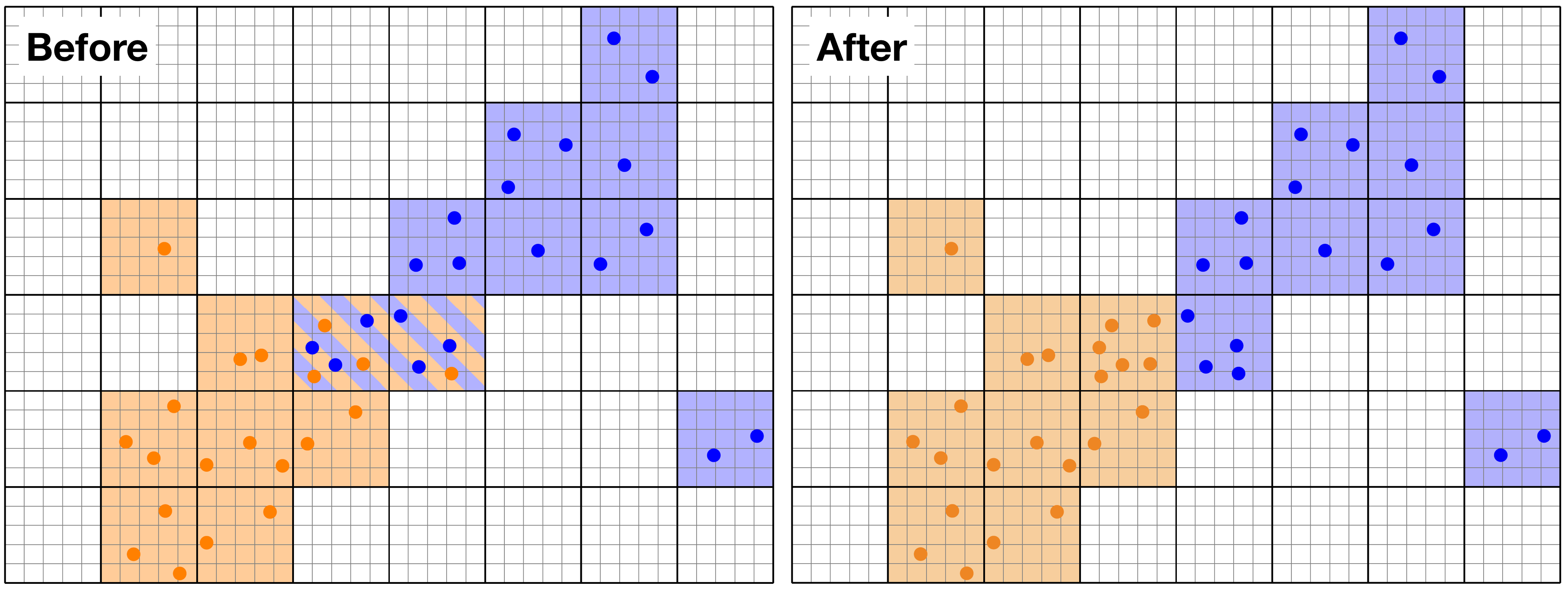 Example of load-balancing for Particles. The domain is chunked along the thick lines, and the orange and blue particles are on separate MPI processors. Before load-balancing (left panel), two chuncks in the centre of the domain have both orange and blue particles. After the load-balancing (right panel), the Particles are redistributed over the processors so that the number of chunks and particles per processor is optimised.
The difficulty is that since we don't know how the ParticleSet will disperse over time, we need to do this load-balancing 'on the fly'. If you to contribute to the optimisation of the load-balancing, please leave a message on github!