Setting up and running absolute hydration free energy calculations
This tutorial gives a step-by-step process to set up absolute hydration free energy (AHFE) simulation campaign using OpenFE. In this tutorial we are performing an absolute hydration free energy calculation of benzene.
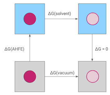
The absolute hydration free energy is obtained through a thermodynamic cycle. The interactions of the molecule are decoupled both in solvent, giving $\Delta G$(solvent) and in vacuum, giving $\Delta G$(vacuum), which allows calculation of the absolute hydration free energy, $\Delta G$(AHFE).
Note: In this protocol, the coulombic interactions of the molecule are fully turned off (annihilated), while the Lennard-Jones interactions are decoupled, meaning the intermolecular interactions turned off, keeping the intramolecular Lennard-Jones interactions.
%matplotlib inline
import openfe
1. Loading the ligand
First we must load the chemical models between which we wish to calculate free energies.
In this example these are initially stored in a molfile (.sdf) containing multiple molecules.
This can be loaded using the SDMolSupplier class from rdkit and passed to openfe.
from rdkit import Chem
supp = Chem.SDMolSupplier("../cookbook/assets/benzene.sdf", removeHs=False)
ligands = [openfe.SmallMoleculeComponent.from_rdkit(mol) for mol in supp]
2. Creating ChemicalSystems
OpenFE describes complex molecular systems as being composed of Components. For example, we have SmallMoleculeComponent for each small molecule in the LigandNetwork. We'll create a SolventComponent to describe the solvent.
The Components are joined in a ChemicalSystem, which describes all the particles in the simulation.
In state A of the hydration free energy protocol, the ligand is fully interacting in the solvent and the ChemicalSystem contains both the ligand and the solvent. In the other endstate, state B, the ligand is fully decoupled in the solvent. Therefore, the ChemicalSystem in state B only contains the solvent.
Note that for AHFE simulations, we are not separately defining the vacuum state, but the protocol creates that based on the solvent states.
# defaults are water with NaCl at 0.15 M
solvent = openfe.SolventComponent()
# In state A the ligand is fully interacting in the solvent
systemA = openfe.ChemicalSystem({
    'ligand': ligands[0],
    'solvent': solvent,
}, name=ligands[0].name)
# In state B the ligand is fully decoupled in the solvent, therefore we are only defining the solvent here
systemB = openfe.ChemicalSystem({'solvent': solvent})
3. Defining the AHFE simulation settings and creating a Protocol
There are various different parameters which can be set to determine how the AHFE simulation will take place.
The easiest way to customize protocol settings is to start with the default settings, and modify them. Many settings carry units with them.
from openfe.protocols.openmm_afe import AbsoluteSolvationProtocol
settings = AbsoluteSolvationProtocol.default_settings()
settings
{'alchemical_settings': {},
 'integrator_settings': {'barostat_frequency': <Quantity(25, 'timestep')>,
                         'constraint_tolerance': 1e-06,
                         'langevin_collision_rate': <Quantity(1.0, '1 / picosecond')>,
                         'n_restart_attempts': 20,
                         'reassign_velocities': False,
                         'remove_com': False,
                         'timestep': <Quantity(4, 'femtosecond')>},
 'lambda_settings': {'lambda_elec': [0.0,
                                     0.25,
                                     0.5,
                                     0.75,
                                     1.0,
                                     1.0,
                                     1.0,
                                     1.0,
                                     1.0,
                                     1.0,
                                     1.0,
                                     1.0,
                                     1.0,
                                     1.0],
                     'lambda_restraints': [0.0,
                                           0.0,
                                           0.0,
                                           0.0,
                                           0.0,
                                           0.0,
                                           0.0,
                                           0.0,
                                           0.0,
                                           0.0,
                                           0.0,
                                           0.0,
                                           0.0,
                                           0.0],
                     'lambda_vdw': [0.0,
                                    0.0,
                                    0.0,
                                    0.0,
                                    0.0,
                                    0.12,
                                    0.24,
                                    0.36,
                                    0.48,
                                    0.6,
                                    0.7,
                                    0.77,
                                    0.85,
                                    1.0]},
 'partial_charge_settings': {'nagl_model': None,
                             'number_of_conformers': None,
                             'off_toolkit_backend': 'ambertools',
                             'partial_charge_method': 'am1bcc'},
 'protocol_repeats': 3,
 'solvation_settings': {'solvent_model': 'tip3p',
                        'solvent_padding': <Quantity(1.2, 'nanometer')>},
 'solvent_engine_settings': {'compute_platform': None},
 'solvent_equil_output_settings': {'checkpoint_interval': <Quantity(250, 'picosecond')>,
                                   'checkpoint_storage_filename': 'checkpoint.chk',
                                   'equil_npt_structure': 'equil_npt_structure.pdb',
                                   'equil_nvt_structure': 'equil_nvt_structure.pdb',
                                   'forcefield_cache': 'db.json',
                                   'log_output': 'equil_simulation.log',
                                   'minimized_structure': 'minimized.pdb',
                                   'output_indices': 'not water',
                                   'preminimized_structure': 'system.pdb',
                                   'production_trajectory_filename': 'production_equil.xtc',
                                   'trajectory_write_interval': <Quantity(20, 'picosecond')>},
 'solvent_equil_simulation_settings': {'equilibration_length': <Quantity(0.2, 'nanosecond')>,
                                       'equilibration_length_nvt': <Quantity(0.1, 'nanosecond')>,
                                       'minimization_steps': 5000,
                                       'production_length': <Quantity(0.5, 'nanosecond')>},
 'solvent_forcefield_settings': {'constraints': 'hbonds',
                                 'forcefields': ['amber/ff14SB.xml',
                                                 'amber/tip3p_standard.xml',
                                                 'amber/tip3p_HFE_multivalent.xml',
                                                 'amber/phosaa10.xml'],
                                 'hydrogen_mass': 3.0,
                                 'nonbonded_cutoff': <Quantity(1.0, 'nanometer')>,
                                 'nonbonded_method': 'PME',
                                 'rigid_water': True,
                                 'small_molecule_forcefield': 'openff-2.0.0'},
 'solvent_output_settings': {'checkpoint_interval': <Quantity(250, 'picosecond')>,
                             'checkpoint_storage_filename': 'solvent_checkpoint.nc',
                             'forcefield_cache': 'db.json',
                             'output_filename': 'solvent.nc',
                             'output_indices': 'not water',
                             'output_structure': 'hybrid_system.pdb'},
 'solvent_simulation_settings': {'early_termination_target_error': <Quantity(0.0, 'kilocalorie_per_mole')>,
                                 'equilibration_length': <Quantity(1.0, 'nanosecond')>,
                                 'minimization_steps': 5000,
                                 'n_replicas': 14,
                                 'production_length': <Quantity(10.0, 'nanosecond')>,
                                 'real_time_analysis_interval': <Quantity(250, 'picosecond')>,
                                 'real_time_analysis_minimum_time': <Quantity(500, 'picosecond')>,
                                 'sampler_method': 'repex',
                                 'sams_flatness_criteria': 'logZ-flatness',
                                 'sams_gamma0': 1.0,
                                 'time_per_iteration': <Quantity(1, 'picosecond')>},
 'thermo_settings': {'ph': None,
                     'pressure': <Quantity(0.986923267, 'standard_atmosphere')>,
                     'redox_potential': None,
                     'temperature': <Quantity(298.15, 'kelvin')>},
 'vacuum_engine_settings': {'compute_platform': None},
 'vacuum_equil_output_settings': {'checkpoint_interval': <Quantity(250, 'picosecond')>,
                                  'checkpoint_storage_filename': 'checkpoint.chk',
                                  'equil_npt_structure': 'equil_structure.pdb',
                                  'equil_nvt_structure': None,
                                  'forcefield_cache': 'db.json',
                                  'log_output': 'equil_simulation.log',
                                  'minimized_structure': 'minimized.pdb',
                                  'output_indices': 'not water',
                                  'preminimized_structure': 'system.pdb',
                                  'production_trajectory_filename': 'production_equil.xtc',
                                  'trajectory_write_interval': <Quantity(20, 'picosecond')>},
 'vacuum_equil_simulation_settings': {'equilibration_length': <Quantity(0.2, 'nanosecond')>,
                                      'equilibration_length_nvt': None,
                                      'minimization_steps': 5000,
                                      'production_length': <Quantity(0.5, 'nanosecond')>},
 'vacuum_forcefield_settings': {'constraints': 'hbonds',
                                'forcefields': ['amber/ff14SB.xml',
                                                'amber/tip3p_standard.xml',
                                                'amber/tip3p_HFE_multivalent.xml',
                                                'amber/phosaa10.xml'],
                                'hydrogen_mass': 3.0,
                                'nonbonded_cutoff': <Quantity(1.0, 'nanometer')>,
                                'nonbonded_method': 'nocutoff',
                                'rigid_water': True,
                                'small_molecule_forcefield': 'openff-2.0.0'},
 'vacuum_output_settings': {'checkpoint_interval': <Quantity(250, 'picosecond')>,
                            'checkpoint_storage_filename': 'vacuum_checkpoint.nc',
                            'forcefield_cache': 'db.json',
                            'output_filename': 'vacuum.nc',
                            'output_indices': 'not water',
                            'output_structure': 'hybrid_system.pdb'},
 'vacuum_simulation_settings': {'early_termination_target_error': <Quantity(0.0, 'kilocalorie_per_mole')>,
                                'equilibration_length': <Quantity(0.5, 'nanosecond')>,
                                'minimization_steps': 5000,
                                'n_replicas': 14,
                                'production_length': <Quantity(2.0, 'nanosecond')>,
                                'real_time_analysis_interval': <Quantity(250, 'picosecond')>,
                                'real_time_analysis_minimum_time': <Quantity(500, 'picosecond')>,
                                'sampler_method': 'repex',
                                'sams_flatness_criteria': 'logZ-flatness',
                                'sams_gamma0': 1.0,
                                'time_per_iteration': <Quantity(1, 'picosecond')>}}
Displaying the default values:
settings.thermo_settings.temperature # Simulation temperature
settings.lambda_settings.lambda_elec # List of floats of lambda values for the electrostatics
[0.0, 0.25, 0.5, 0.75, 1.0, 1.0, 1.0, 1.0, 1.0, 1.0, 1.0, 1.0, 1.0, 1.0]
settings.solvent_simulation_settings.equilibration_length # Length of the NPT equilibration in the solvent, prior to running the AHFE calculation
By default we run 3 repeats with solvent and vacuum simulation lengths of 10 ns and 2 ns over 14 lambda windows. To speed things up here we instead run 1 repeat with both solvent and vacuum simulation lengths of 0.5 ns over 14 lambda windows.
Changing default values:
from openff.units import unit

# change the values
settings.protocol_repeats = 1
settings.lambda_settings.lambda_elec = [0.0, 0.26, 0.5, 0.75, 1.0, 1.0, 1.0, 1.0, 1.0, 1.0, 1.0, 1.0, 1.0, 1.0]
settings.solvent_simulation_settings.equilibration_length = 10 * unit.picosecond
settings.solvent_simulation_settings.production_length = 500 * unit.picosecond
settings.vacuum_simulation_settings.equilibration_length = 10 * unit.picosecond
settings.vacuum_simulation_settings.production_length = 500 * unit.picosecond
settings.solvent_engine_settings.compute_platform = 'CUDA'
Here a view of all the settings that the user can modify as shown in the examples above:
settings
{'alchemical_settings': {},
 'integrator_settings': {'barostat_frequency': <Quantity(25, 'timestep')>,
                         'constraint_tolerance': 1e-06,
                         'langevin_collision_rate': <Quantity(1.0, '1 / picosecond')>,
                         'n_restart_attempts': 20,
                         'reassign_velocities': False,
                         'remove_com': False,
                         'timestep': <Quantity(4, 'femtosecond')>},
 'lambda_settings': {'lambda_elec': [0.0,
                                     0.26,
                                     0.5,
                                     0.75,
                                     1.0,
                                     1.0,
                                     1.0,
                                     1.0,
                                     1.0,
                                     1.0,
                                     1.0,
                                     1.0,
                                     1.0,
                                     1.0],
                     'lambda_restraints': [0.0,
                                           0.0,
                                           0.0,
                                           0.0,
                                           0.0,
                                           0.0,
                                           0.0,
                                           0.0,
                                           0.0,
                                           0.0,
                                           0.0,
                                           0.0,
                                           0.0,
                                           0.0],
                     'lambda_vdw': [0.0,
                                    0.0,
                                    0.0,
                                    0.0,
                                    0.0,
                                    0.12,
                                    0.24,
                                    0.36,
                                    0.48,
                                    0.6,
                                    0.7,
                                    0.77,
                                    0.85,
                                    1.0]},
 'partial_charge_settings': {'nagl_model': None,
                             'number_of_conformers': None,
                             'off_toolkit_backend': 'ambertools',
                             'partial_charge_method': 'am1bcc'},
 'protocol_repeats': 1,
 'solvation_settings': {'solvent_model': 'tip3p',
                        'solvent_padding': <Quantity(1.2, 'nanometer')>},
 'solvent_engine_settings': {'compute_platform': 'CUDA'},
 'solvent_equil_output_settings': {'checkpoint_interval': <Quantity(250, 'picosecond')>,
                                   'checkpoint_storage_filename': 'checkpoint.chk',
                                   'equil_npt_structure': 'equil_npt_structure.pdb',
                                   'equil_nvt_structure': 'equil_nvt_structure.pdb',
                                   'forcefield_cache': 'db.json',
                                   'log_output': 'equil_simulation.log',
                                   'minimized_structure': 'minimized.pdb',
                                   'output_indices': 'not water',
                                   'preminimized_structure': 'system.pdb',
                                   'production_trajectory_filename': 'production_equil.xtc',
                                   'trajectory_write_interval': <Quantity(20, 'picosecond')>},
 'solvent_equil_simulation_settings': {'equilibration_length': <Quantity(0.2, 'nanosecond')>,
                                       'equilibration_length_nvt': <Quantity(0.1, 'nanosecond')>,
                                       'minimization_steps': 5000,
                                       'production_length': <Quantity(0.5, 'nanosecond')>},
 'solvent_forcefield_settings': {'constraints': 'hbonds',
                                 'forcefields': ['amber/ff14SB.xml',
                                                 'amber/tip3p_standard.xml',
                                                 'amber/tip3p_HFE_multivalent.xml',
                                                 'amber/phosaa10.xml'],
                                 'hydrogen_mass': 3.0,
                                 'nonbonded_cutoff': <Quantity(1.0, 'nanometer')>,
                                 'nonbonded_method': 'PME',
                                 'rigid_water': True,
                                 'small_molecule_forcefield': 'openff-2.0.0'},
 'solvent_output_settings': {'checkpoint_interval': <Quantity(250, 'picosecond')>,
                             'checkpoint_storage_filename': 'solvent_checkpoint.nc',
                             'forcefield_cache': 'db.json',
                             'output_filename': 'solvent.nc',
                             'output_indices': 'not water',
                             'output_structure': 'hybrid_system.pdb'},
 'solvent_simulation_settings': {'early_termination_target_error': <Quantity(0.0, 'kilocalorie_per_mole')>,
                                 'equilibration_length': <Quantity(0.01, 'nanosecond')>,
                                 'minimization_steps': 5000,
                                 'n_replicas': 14,
                                 'production_length': <Quantity(0.5, 'nanosecond')>,
                                 'real_time_analysis_interval': <Quantity(250, 'picosecond')>,
                                 'real_time_analysis_minimum_time': <Quantity(500, 'picosecond')>,
                                 'sampler_method': 'repex',
                                 'sams_flatness_criteria': 'logZ-flatness',
                                 'sams_gamma0': 1.0,
                                 'time_per_iteration': <Quantity(1, 'picosecond')>},
 'thermo_settings': {'ph': None,
                     'pressure': <Quantity(0.986923267, 'standard_atmosphere')>,
                     'redox_potential': None,
                     'temperature': <Quantity(298.15, 'kelvin')>},
 'vacuum_engine_settings': {'compute_platform': None},
 'vacuum_equil_output_settings': {'checkpoint_interval': <Quantity(250, 'picosecond')>,
                                  'checkpoint_storage_filename': 'checkpoint.chk',
                                  'equil_npt_structure': 'equil_structure.pdb',
                                  'equil_nvt_structure': None,
                                  'forcefield_cache': 'db.json',
                                  'log_output': 'equil_simulation.log',
                                  'minimized_structure': 'minimized.pdb',
                                  'output_indices': 'not water',
                                  'preminimized_structure': 'system.pdb',
                                  'production_trajectory_filename': 'production_equil.xtc',
                                  'trajectory_write_interval': <Quantity(20, 'picosecond')>},
 'vacuum_equil_simulation_settings': {'equilibration_length': <Quantity(0.2, 'nanosecond')>,
                                      'equilibration_length_nvt': None,
                                      'minimization_steps': 5000,
                                      'production_length': <Quantity(0.5, 'nanosecond')>},
 'vacuum_forcefield_settings': {'constraints': 'hbonds',
                                'forcefields': ['amber/ff14SB.xml',
                                                'amber/tip3p_standard.xml',
                                                'amber/tip3p_HFE_multivalent.xml',
                                                'amber/phosaa10.xml'],
                                'hydrogen_mass': 3.0,
                                'nonbonded_cutoff': <Quantity(1.0, 'nanometer')>,
                                'nonbonded_method': 'nocutoff',
                                'rigid_water': True,
                                'small_molecule_forcefield': 'openff-2.0.0'},
 'vacuum_output_settings': {'checkpoint_interval': <Quantity(250, 'picosecond')>,
                            'checkpoint_storage_filename': 'vacuum_checkpoint.nc',
                            'forcefield_cache': 'db.json',
                            'output_filename': 'vacuum.nc',
                            'output_indices': 'not water',
                            'output_structure': 'hybrid_system.pdb'},
 'vacuum_simulation_settings': {'early_termination_target_error': <Quantity(0.0, 'kilocalorie_per_mole')>,
                                'equilibration_length': <Quantity(0.01, 'nanosecond')>,
                                'minimization_steps': 5000,
                                'n_replicas': 14,
                                'production_length': <Quantity(0.5, 'nanosecond')>,
                                'real_time_analysis_interval': <Quantity(250, 'picosecond')>,
                                'real_time_analysis_minimum_time': <Quantity(500, 'picosecond')>,
                                'sampler_method': 'repex',
                                'sams_flatness_criteria': 'logZ-flatness',
                                'sams_gamma0': 1.0,
                                'time_per_iteration': <Quantity(1, 'picosecond')>}}
Creating the Protocol
With the Settings inspected and adjusted, we can provide these to the Protocol. This Protocol defines the procedure to estimate a free energy difference between two chemical systems, with the details of the two end states yet to be defined.
protocol = AbsoluteSolvationProtocol(settings=settings)
4. Running the AHFE simulation
(a) Using the CLI
Once we have the ChemicalSystems, and the Protocol, we can create the Transformation.
transformation = openfe.Transformation(
            stateA=systemA,
            stateB=systemB,
            mapping=None,
            protocol=protocol,  # use protocol created above
            name=f"{systemA.name}"
        )
We'll write out the transformation to disk, so that it can be run using the openfe quickrun command:
import pathlib
# first we create the directory
transformation_dir = pathlib.Path("ahfe_json")
transformation_dir.mkdir(exist_ok=True)

# then we write out the transformation
transformation.dump(transformation_dir / f"{transformation.name}.json")
You can run the AHFE simulation from the CLI by using the openfe quickrun command. It takes a transformation JSON as input, and the flags -o to give the final output JSON file and -d for the directory where simulation results should be stored. For example,
openfe quickrun path/to/transformation.json -o results.json -d working-directory
where path/to/transformation.json is the path to one of the files created above.
(b) Using the Python API
Creating the ProtocolDAG
Once we have the two ChemicalSystems, and the Protocol, we can create the ProtocolDAG.
This creates a directed-acyclic-graph (DAG) of computational tasks necessary for creating an estimate of the free energy difference between the two chemical systems.
dag = protocol.create(stateA=systemA, stateB=systemB, mapping=None)
To summarize, this ProtocolDAG contains:
- chemical models of both sides of the alchemical transformation in
systemAandsystemB - a description of the exact computational algorithm to use to perform the estimate in
protocol - the
mappingis set toNonesince no atoms are mapped in the AHFE protocol
Executing the simulation
The DAG contains many invdividual jobs. We can execute them sequentially in this notebook using the gufe.protocols.execute function.
In a more realistic (expansive) situation we would farm off the individual jobs to a HPC cluster or cloud compute service so they could be executed in parallel.
Note: we use the shared_basedir and scratch_basedir argument of execute_DAG in order to set the directory where the simulation files are written to
from gufe.protocols import execute_DAG
import pathlib
# Finally we can run the simulations
path = pathlib.Path('./ahfe_results')
path.mkdir()

# Execute the DAG
dag_results = execute_DAG(dag, scratch_basedir=path, shared_basedir=path, n_retries=3)
/Users/hannahbaumann/openfe/openfe/protocols/openmm_rfe/_rfe_utils/compute.py:56: UserWarning: Non-GPU platform selected: CPU, this may significantly impact simulation performance
  warnings.warn(wmsg)
WARNING:root:Non-GPU platform selected: CPU, this may significantly impact simulation performance
WARNING:openmmtools.multistate.multistatereporter:Warning: The openmmtools.multistate API is experimental and may change in future releases
WARNING:root:Non-GPU platform selected: CPU, this may significantly impact simulation performance
WARNING:openmmtools.multistate.multistatesampler:Warning: The openmmtools.multistate API is experimental and may change in future releases
Please cite the following:

        Friedrichs MS, Eastman P, Vaidyanathan V, Houston M, LeGrand S, Beberg AL, Ensign DL, Bruns CM, and Pande VS. Accelerating molecular dynamic simulations on graphics processing unit. J. Comput. Chem. 30:864, 2009. DOI: 10.1002/jcc.21209
        Eastman P and Pande VS. OpenMM: A hardware-independent framework for molecular simulations. Comput. Sci. Eng. 12:34, 2010. DOI: 10.1109/MCSE.2010.27
        Eastman P and Pande VS. Efficient nonbonded interactions for molecular dynamics on a graphics processing unit. J. Comput. Chem. 31:1268, 2010. DOI: 10.1002/jcc.21413
        Eastman P and Pande VS. Constant constraint matrix approximation: A robust, parallelizable constraint method for molecular simulations. J. Chem. Theor. Comput. 6:434, 2010. DOI: 10.1021/ct900463w
        Chodera JD and Shirts MR. Replica exchange and expanded ensemble simulations as Gibbs multistate: Simple improvements for enhanced mixing. J. Chem. Phys., 135:194110, 2011. DOI:10.1063/1.3660669
6. Analysis
Finally now that we've run our simulations, let's go ahead and gather the free energies for both phases.
Python API
If you executed the simulations using the Python API, you will have generated a dag_results object. You can analyze these results by calling the Protocols' gather() method. This takes a list of completed DAG results and returns a AbsoluteSolvationProtocolResult which can return a free energy estimate and uncertainty by calling the get_estimate() and get_uncertainty() methods.
# Get the complex and solvent results
protocol_results = protocol.gather([dag_results])

print(f"AHFE dG: {protocol_results.get_estimate()}, err {protocol_results.get_uncertainty()}")
You can save the AbsoluteSolvationProtocolResult to a JSON output file in the following manner:
# Save the results in a json file
import gzip
import json
import gufe
outdict = {
    "estimate": protocol_results.get_estimate(),
    "uncertainty": protocol_results.get_uncertainty(),
    "protocol_result": protocol_results.to_dict(),
    "unit_results": {
        unit.key: unit.to_keyed_dict()
        for unit in dag_results.protocol_unit_results
    }
}

with open("ahfe_json/benzene_results.json") as stream:
    json.dump(outdict, stream, cls=gufe.tokenization.JSON_HANDLER.encoder)
CLI / Quickrun
If you ran the simulation using the CLI (i.e. by calling openfe quickrun ) you will end up with the same JSON output file as the one created in the previous cell. To get your simulation results you can load them back into Python in the following manner:
import gzip
import json
import gufe

outfile = "ahfe_json/benzene_results.json"
with open(outfile) as stream:
    results = json.load(stream)
    estimate = results['estimate']
    uncertainty = results['uncertainty']
estimate
{'magnitude': -0.7536190151704971,
 'unit': 'kilocalorie_per_mole',
 ':is_custom:': True,
 'pint_unit_registry': 'openff_units'}