Optimal Transport

Optimal Transport¶

Overview¶

The transportation or optimal transport problem is interesting both because of its many applications and because of its important role in the history of economic theory.

In this lecture, we describe the problem, tell how linear programming is a key tool for solving it, and then provide some examples.

We will provide other applications in followup lectures.

The optimal transport problem was studied in early work about linear programming, as summarized for example by [Dorfman et al., 1958]. A modern reference about applications in economics is [Galichon, 2016].

Below, we show how to solve the optimal transport problem using several implementations of linear programming, including, in order,

linprog solver from SciPy,

the linprog_simplex solver from QuantEcon and
the simplex-based solvers included in the Python Optimal Transport package.

In [ ]:

!pip install --upgrade quantecon
!pip install --upgrade POT

Let’s start with some imports.

In [ ]:

import numpy as np
import matplotlib.pyplot as plt
from scipy.optimize import linprog
from quantecon.optimize.linprog_simplex import linprog_simplex
import ot
from scipy.stats import betabinom
import networkx as nx

The Optimal Transport Problem¶

Suppose that $ m $ factories produce goods that must be sent to $ n $ locations.

Let

$ x_{ij} $ denote the quantity shipped from factory $ i $ to location $ j $
$ c_{ij} $ denote the cost of shipping one unit from factory $ i $ to location $ j $
$ p_i $ denote the capacity of factory $ i $ and $ q_j $ denote the amount required at location $ j $.
$ i = 1, 2, \dots, m $ and $ j = 1, 2, \dots, n $.

A planner wants to minimize total transportation costs subject to the following constraints:

The amount shipped from each factory must equal its capacity.
The amount shipped to each location must equal the quantity required there.

The figure below shows one visualization of this idea, when factories and target locations are distributed in the plane.

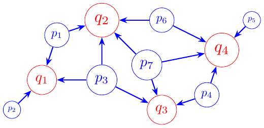
The size of the vertices in the figure are proportional to

capacity, for the factories, and
demand (amount required) for the target locations.

The arrows show one possible transport plan, which respects the constraints stated above.

The planner’s problem can be expressed as the following constrained minimization problem:

$$ \begin{aligned} \min_{x_{ij}} \ & \sum_{i=1}^m \sum_{j=1}^n c_{ij} x_{ij} \\ \mbox{subject to } \ & \sum_{j=1}^n x_{ij} = p_i, & i = 1, 2, \dots, m \\ & \sum_{i=1}^m x_{ij} = q_j, & j = 1, 2, \dots, n \\ & x_{ij} \ge 0 \\ \end{aligned} \tag{17.1} $$

This is an optimal transport problem with

$ mn $ decision variables, namely, the entries $ x_{ij} $ and
$ m+n $ constraints.

Summing the $ q_j $’s across all $ j $’s and the $ p_i $’s across all $ i $’s indicates that the total capacity of all the factories equals total requirements at all locations:

$$ \sum_{j=1}^n q_j = \sum_{j=1}^n \sum_{i=1}^m x_{ij} = \sum_{i=1}^m \sum_{j=1}^n x_{ij} = \sum_{i=1}^m p_i \tag{17.2} $$

The presence of the restrictions in (17.2) will be the source of one redundancy in the complete set of restrictions that we describe below.

More about this later.

The Linear Programming Approach¶

In this section we discuss using using standard linear programming solvers to tackle the optimal transport problem.

Vectorizing a Matrix of Decision Variables¶

A matrix of decision variables $ x_{ij} $ appears in problem (17.1).

The SciPy function linprog expects to see a vector of decision variables.

This situation impels us to rewrite our problem in terms of a vector of decision variables.

Let

$ X, C $ be $ m \times n $ matrices with entries $ x_{ij}, c_{ij} $,
$ p $ be $ m $-dimensional vector with entries $ p_i $,
$ q $ be $ n $-dimensional vector with entries $ q_j $.

With $ \mathbf{1}_n $ denoting the $ n $-dimensional column vector $ (1, 1, \dots, 1)' $, our problem can now be expressed compactly as:

$$ \begin{aligned} \min_{X} \ & \operatorname{tr} (C' X) \\ \mbox{subject to } \ & X \ \mathbf{1}_n = p \\ & X' \ \mathbf{1}_m = q \\ & X \ge 0 \\ \end{aligned} $$

We can convert the matrix $ X $ into a vector by stacking all of its columns into a column vector.

Doing this is called vectorization, an operation that we denote $ \operatorname{vec}(X) $.

Similarly, we convert the matrix $ C $ into an $ mn $-dimensional vector $ \operatorname{vec}(C) $.

The objective function can be expressed as the inner product between $ \operatorname{vec}(C) $ and $ \operatorname{vec}(X) $:

$$ \operatorname{vec}(C)' \cdot \operatorname{vec}(X). $$

To express the constraints in terms of $ \operatorname{vec}(X) $, we use a Kronecker product denoted by $ \otimes $ and defined as follows.

Suppose $ A $ is an $ m \times s $ matrix with entries $ (a_{ij}) $ and that $ B $ is an $ n \times t $ matrix.

The Kronecker product of $ A $ and $ B $ is defined, in block matrix form, by

$$ A \otimes B = \begin{pmatrix} a_{11}B & a_{12}B & \dots & a_{1s}B \\ a_{21}B & a_{22}B & \dots & a_{2s}B \\ & & \vdots & \\ a_{m1}B & a_{m2}B & \dots & a_{ms}B \\ \end{pmatrix}. $$

$ A \otimes B $ is an $ mn \times st $ matrix.

It has the property that for any $ m \times n $ matrix $ X $

$$ \operatorname{vec}(A'XB) = (B' \otimes A') \operatorname{vec}(X). \tag{17.3} $$

We can now express our constraints in terms of $ \operatorname{vec}(X) $.

Let $ A = \mathbf{I}_m', B = \mathbf{1}_n $.

By equation (17.3)

$$ X \ \mathbf{1}_n = \operatorname{vec}(X \ \mathbf{1}_n) = \operatorname{vec}(\mathbf{I}_m X \ \mathbf{1}_n) = (\mathbf{1}_n' \otimes \mathbf{I}_m) \operatorname{vec}(X). $$

where $ \mathbf{I}_m $ denotes the $ m \times m $ identity matrix.

Constraint $ X \ \mathbf{1}_n = p $ can now be written as:

$$ (\mathbf{1}_n' \otimes \mathbf{I}_m) \operatorname{vec}(X) = p. $$

Similarly, the constraint $ X' \ \mathbf{1}_m = q $ can be rewriten as:

$$ (\mathbf{I}_n \otimes \mathbf{1}_m') \operatorname{vec}(X) = q. $$

With $ z := \operatorname{vec}(X) $, our problem can now be expressed in terms of an $ mn $-dimensional vector of decision variables:

$$ \begin{aligned} \min_{z} \ & \operatorname{vec}(C)' z \\ \mbox{subject to } \ & A z = b \\ & z \ge 0 \\ \end{aligned} \tag{17.4} $$

where

$$ A = \begin{pmatrix} \mathbf{1}_n' \otimes \mathbf{I}_m \\ \mathbf{I}_n \otimes \mathbf{1}_m' \\ \end{pmatrix} \quad \text{and} \quad b = \begin{pmatrix} p \\ q \\ \end{pmatrix} $$

An Application¶

We now provide an example that takes the form (17.4) that we’ll solve by deploying the function linprog.

The table below provides numbers for the requirements vector $ q $, the capacity vector $ p $, and entries $ c_{ij} $ of the cost-of-shipping matrix $ C $.

The numbers in the above table tell us to set $ m = 3 $, $ n = 5 $, and construct the following objects:

$$ p = \begin{pmatrix} 50 \\ 100 \\ 150 \end{pmatrix}, \quad q = \begin{pmatrix} 25 \\ 115 \\ 60 \\ 30 \\ 70 \end{pmatrix} \quad \text{and} \quad C = \begin{pmatrix} 10 &15 &20 &20 &40 \\ 20 &40 &15 &30 &30 \\ 30 &35 &40 &55 &25 \end{pmatrix}. $$

Let’s write Python code that sets up the problem and solves it.

In [ ]:

# Define parameters
m = 3
n = 5

p = np.array([50, 100, 150])
q = np.array([25, 115, 60, 30, 70])

C = np.array([[10, 15, 20, 20, 40],
              [20, 40, 15, 30, 30],
              [30, 35, 40, 55, 25]])

# Vectorize matrix C
C_vec = C.reshape((m*n, 1), order='F')

# Construct matrix A by Kronecker product
A1 = np.kron(np.ones((1, n)), np.identity(m))
A2 = np.kron(np.identity(n), np.ones((1, m)))
A = np.vstack([A1, A2])

# Construct vector b
b = np.hstack([p, q])

# Solve the primal problem
res = linprog(C_vec, A_eq=A, b_eq=b)

# Print results
print("message:", res.message)
print("nit:", res.nit)
print("fun:", res.fun)
print("z:", res.x)
print("X:", res.x.reshape((m,n), order='F'))

Notice how, in the line C_vec = C.reshape((m*n, 1), order='F'), we are careful to vectorize using the flag order='F'.

This is consistent with converting $ C $ into a vector by stacking all of its columns into a column vector.

Here 'F' stands for “Fortran”, and we are using Fortran style column-major order.

(For an alternative approach, using Python’s default row-major ordering, see this lecture by Alfred Galichon.)

Interpreting the warning:

The above warning message from SciPy points out that A is not full rank.

This indicates that the linear program has been set up to include one or more redundant constraints.

Here, the source of the redundancy is the structure of restrictions (17.2).

Let’s explore this further by printing out $ A $ and staring at it.

In [ ]:

The singularity of $ A $ reflects that the first three constraints and the last five constraints both require that “total requirements equal total capacities” expressed in (17.2).

One equality constraint here is redundant.

Below we drop one of the equality constraints, and use only 7 of them.

After doing this, we attain the same minimized cost.

However, we find a different transportation plan.

Though it is a different plan, it attains the same cost!

In [ ]:

linprog(C_vec, A_eq=A[:-1], b_eq=b[:-1])

In [ ]:

%time linprog(C_vec, A_eq=A[:-1], b_eq=b[:-1])

In [ ]:

%time linprog(C_vec, A_eq=A, b_eq=b)

Evidently, it is slightly quicker to work with the system that removed a redundant constraint.

Let’s drill down and do some more calculations to help us understand whether or not our finding two different optimal transport plans reflects our having dropped a redundant equality constraint.

Hint¶

It will turn out that dropping a redundant equality isn’t really what mattered.

To verify our hint, we shall simply use all of the original equality constraints (including a redundant one), but we’ll just shuffle the order of the constraints.

In [ ]:

arr = np.arange(m+n)

In [ ]:

sol_found = []
cost = []

# simulate 1000 times
for i in range(1000):

    np.random.shuffle(arr)
    res_shuffle = linprog(C_vec, A_eq=A[arr], b_eq=b[arr])

    # if find a new solution
    sol = tuple(res_shuffle.x)
    if sol not in sol_found:
        sol_found.append(sol)
        cost.append(res_shuffle.fun)

In [ ]:

for i in range(len(sol_found)):
    print(f"transportation plan {i}: ", sol_found[i])
    print(f"     minimized cost {i}: ", cost[i])

Ah hah! As you can see, putting constraints in different orders in this case uncovers two optimal transportation plans that achieve the same minimized cost.

These are the same two plans computed earlier.

Next, we show that leaving out the first constraint “accidentally” leads to the initial plan that we computed.

In [ ]:

linprog(C_vec, A_eq=A[1:], b_eq=b[1:])

Let’s compare this transport plan with

In [ ]:

res.x

Here the matrix $ X $ contains entries $ x_{ij} $ that tell amounts shipped from factor $ i = 1, 2, 3 $ to location $ j=1,2, \ldots, 5 $.

The vector $ z $ evidently equals $ \operatorname{vec}(X) $.

The minimized cost from the optimal transport plan is given by the $ fun $ variable.

Using a Just-in-Time Compiler¶

We can also solve optimal transportation problems using a powerful tool from QuantEcon, namely, quantecon.optimize.linprog_simplex.

While this routine uses the same simplex algorithm as scipy.optimize.linprog, the code is accelerated by using a just-in-time compiler shipped in the numba library.

As you will see very soon, by using scipy.optimize.linprog the time required to solve an optimal transportation problem can be reduced significantly.

In [ ]:

# construct matrices/vectors for linprog_simplex
c = C.flatten()

# Equality constraints
A_eq = np.zeros((m+n, m*n))
for i in range(m):
    for j in range(n):
        A_eq[i, i*n+j] = 1
        A_eq[m+j, i*n+j] = 1

b_eq = np.hstack([p, q])

Since quantecon.optimize.linprog_simplex does maximization instead of minimization, we need to put a negative sign before vector c.

In [ ]:

res_qe = linprog_simplex(-c, A_eq=A_eq, b_eq=b_eq)

Since the two LP solvers use the same simplex algorithm, we expect to get exactly the same solutions

In [ ]:

res_qe.x.reshape((m, n), order='C')

In [ ]:

res.x.reshape((m, n), order='F')

Let’s do a speed comparison between scipy.optimize.linprog and quantecon.optimize.linprog_simplex.

In [ ]:

# scipy.optimize.linprog
%time res = linprog(C_vec, A_eq=A[:-1, :], b_eq=b[:-1])

In [ ]:

# quantecon.optimize.linprog_simplex
%time out = linprog_simplex(-c, A_eq=A_eq, b_eq=b_eq)

As you can see, the quantecon.optimize.linprog_simplex is much faster.

(Note however, that the SciPy version is probably more stable than the QuantEcon version, having been tested more extensively over a longer period of time.)

The Dual Problem¶

Let $ u, v $ denotes vectors of dual decision variables with entries $ (u_i), (v_j) $.

The dual to minimization problem (17.1) is the maximization problem:

$$ \begin{aligned} \max_{u_i, v_j} \ & \sum_{i=1}^m p_i u_i + \sum_{j=1}^n q_j v_j \\ \mbox{subject to } \ & u_i + v_j \le c_{ij}, \ i = 1, 2, \dots, m;\ j = 1, 2, \dots, n \\ \end{aligned} \tag{17.5} $$

The dual problem is also a linear programming problem.

It has $ m+n $ dual variables and $ mn $ constraints.

Vectors $ u $ and $ v $ of values are attached to the first and the second sets of primal constraits, respectively.

Thus, $ u $ is attached to the constraints

$ (\mathbf{1}_n' \otimes \mathbf{I}_m) \operatorname{vec}(X) = p $

and $ v $ is attached to constraints

$ (\mathbf{I}_n \otimes \mathbf{1}_m') \operatorname{vec}(X) = q. $

Components of the vectors $ u $ and $ v $ of per unit values are shadow prices of the quantities appearing on the right sides of those constraints.

We can write the dual problem as

$$ \begin{aligned} \max_{u_i, v_j} \ & p u + q v \\ \mbox{subject to } \ & A' \begin{pmatrix} u \\ v \\ \end{pmatrix} = \operatorname{vec}(C) \\ \end{aligned} \tag{17.6} $$

For the same numerical example described above, let’s solve the dual problem.

In [ ]:

# Solve the dual problem
res_dual = linprog(-b, A_ub=A.T, b_ub=C_vec,
                   bounds=[(None, None)]*(m+n))

#Print results
print("message:", res_dual.message)
print("nit:", res_dual.nit)
print("fun:", res_dual.fun)
print("u:", res_dual.x[:m])
print("v:", res_dual.x[-n:])

We can also solve the dual problem using quantecon.optimize.linprog_simplex.

In [ ]:

res_dual_qe = linprog_simplex(b_eq, A_ub=A_eq.T, b_ub=c)

And the shadow prices computed by the two programs are identical.

In [ ]:

res_dual_qe.x

In [ ]:

res_dual.x

We can compare computational times from using our two tools.

In [ ]:

%time linprog(-b, A_ub=A.T, b_ub=C_vec, bounds=[(None, None)]*(m+n))

In [ ]:

%time linprog_simplex(b_eq, A_ub=A_eq.T, b_ub=c)

quantecon.optimize.linprog_simplex solves the dual problem 10 times faster.

Just for completeness, let’s solve the dual problems with nonsingular $ A $ matrices that we create by dropping a redundant equality constraint.

Try first leaving out the first constraint:

In [ ]:

linprog(-b[1:], A_ub=A[1:].T, b_ub=C_vec,
        bounds=[(None, None)]*(m+n-1))

Not let’s instead leave out the last constraint:

In [ ]:

linprog(-b[:-1], A_ub=A[:-1].T, b_ub=C_vec,
        bounds=[(None, None)]*(m+n-1))

Interpretation of dual problem¶

By strong duality (please see this lecture Linear Programming), we know that:

$$ \sum_{i=1}^m \sum_{j=1}^n c_{ij} x_{ij} = \sum_{i=1}^m p_i u_i + \sum_{j=1}^n q_j v_j $$

One unit more capacity in factory $ i $, i.e. $ p_i $, results in $ u_i $ more transportation costs.

Thus, $ u_i $ describes the cost of shipping one unit from factory $ i $.

Call this the ship-out cost of one unit shipped from factory $ i $.

Similarly, $ v_j $ is the cost of shipping one unit to location $ j $.

Call this the ship-in cost of one unit to location $ j $.

Strong duality implies that total transprotation costs equals total ship-out costs plus total ship-in costs.

It is reasonable that, for one unit of a product, ship-out cost $ u_i $ plus ship-in cost $ v_j $ should equal transportation cost $ c_{ij} $.

This equality is assured by complementary slackness conditions that state that whenever $ x_{ij} > 0 $, meaning that there are positive shipments from factory $ i $ to location $ j $, it must be true that $ u_i + v_j = c_{ij} $.

The Python Optimal Transport Package¶

There is an excellent Python package for optimal transport that simplifies some of the steps we took above.

In particular, the package takes care of the vectorization steps before passing the data out to a linear programming routine.

(That said, the discussion provided above on vectorization remains important, since we want to understand what happens under the hood.)

Replicating Previous Results¶

The following line of code solves the example application discussed above using linear programming.

In [ ]:

X = ot.emd(p, q, C)
X

Sure enough, we have the same solution and the same cost

In [ ]:

total_cost = np.sum(X * C)
total_cost

A Larger Application¶

Now let’s try using the same package on a slightly larger application.

The application has the same interpretation as above but we will also give each node (i.e., vertex) a location in the plane.

This will allow us to plot the resulting transport plan as edges in a graph.

The following class defines a node by

its location $ (x, y) \in \mathbb R^2 $,
its group (factory or location, denoted by p or q) and
its mass (e.g., $ p_i $ or $ q_j $).

In [ ]:

class Node:

    def __init__(self, x, y, mass, group, name):

        self.x, self.y = x, y
        self.mass, self.group = mass, group
        self.name = name

Next we write a function that repeatedly calls the class above to build instances.

It allocates to the nodes it creates their location, mass, and group.

Locations are assigned randomly.

In [ ]:

def build_nodes_of_one_type(group='p', n=100, seed=123):

    nodes = []
    np.random.seed(seed)

    for i in range(n):

        if group == 'p':
            m = 1/n
            x = np.random.uniform(-2, 2)
            y = np.random.uniform(-2, 2)
        else:
            m = betabinom.pmf(i, n-1, 2, 2)
            x = 0.6 * np.random.uniform(-1.5, 1.5)
            y = 0.6 * np.random.uniform(-1.5, 1.5)

        name = group + str(i)
        nodes.append(Node(x, y, m, group, name))

    return nodes

Now we build two lists of nodes, each one containing one type (factories or locations)

In [ ]:

n_p = 32
n_q = 32
p_list = build_nodes_of_one_type(group='p', n=n_p)
q_list = build_nodes_of_one_type(group='q', n=n_q)

p_probs = [p.mass for p in p_list]
q_probs = [q.mass for q in q_list]

For the cost matrix $ C $, we use the Euclidean distance between each factory and location.

In [ ]:

c = np.empty((n_p, n_q))
for i in range(n_p):
    for j in range(n_q):
        x0, y0 = p_list[i].x, p_list[i].y
        x1, y1 = q_list[j].x, q_list[j].y
        c[i, j] = np.sqrt((x0-x1)**2 + (y0-y1)**2)

Now we are ready to apply the solver

In [ ]:

%time pi = ot.emd(p_probs, q_probs, c)

Finally, let’s plot the results using networkx.

In the plot below,

node size is proportional to probability mass
an edge (arrow) from $ i $ to $ j $ is drawn when a positive transfer is made from $ i $ to $ j $ under the optimal transport plan.

In [ ]:

g = nx.DiGraph()
g.add_nodes_from([p.name for p in p_list])
g.add_nodes_from([q.name for q in q_list])

for i in range(n_p):
    for j in range(n_q):
        if pi[i, j] > 0:
            g.add_edge(p_list[i].name, q_list[j].name, weight=pi[i, j])

node_pos_dict={}
for p in p_list:
    node_pos_dict[p.name] = (p.x, p.y)

for q in q_list:
    node_pos_dict[q.name] = (q.x, q.y)

node_color_list = []
node_size_list = []
scale = 8_000
for p in p_list:
    node_color_list.append('blue')
    node_size_list.append(p.mass * scale)
for q in q_list:
    node_color_list.append('red')
    node_size_list.append(q.mass * scale)


fig, ax = plt.subplots(figsize=(7, 10))
plt.axis('off')

nx.draw_networkx_nodes(g,
                       node_pos_dict,
                       node_color=node_color_list,
                       node_size=node_size_list,
                       edgecolors='grey',
                       linewidths=1,
                       alpha=0.5,
                       ax=ax)

nx.draw_networkx_edges(g,
                       node_pos_dict,
                       arrows=True,
                       connectionstyle='arc3,rad=0.1',
                       alpha=0.6)
plt.show()