IPython in action creating reproducible and publishable interactive work.

What is this?¶

This repo contains the complete talk I intend to deliver (have delivered) at PyConZA2013. It contains all the files needed to build a final publishable PDF document from an interactive notebook and even adds a custom front page.

The Complete Talk GitHub Website can be accessed here

Background¶

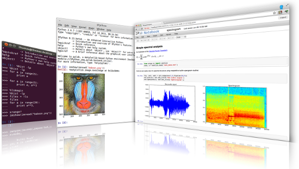
IPython had become a popular choice for doing interactive scientific work. It extends the standard Python interpreter and adds many useful new futures. There is really no need to use the standard Python interpreter anymore. In addition to this IPython offers a web based Notebook that makes interactive work much easier, and have been used to write repeatable scientific papers and more recently a book has been written using this platform, the online Notebook Viewer and GitHub. The development of this material and tool chain to compile the notebook to a publishable PDF, has inspired me to maybe even try and turn this into a complete (free) book. Let’s see what happens.

Combining the most common scientific packages with IPython makes it a formidable tool and serious competition to R. ( R is still awesome! )

As a matter of fact you can run R in the notebook session, embed YouTube Videos, Images and lots more but let me not get ahead of myself....

The science stack consists of (but not limited to):

package	description
pandas	`dataframe` implementation (based on numpy)
scipy	efficient numerical routines
sympy	`symbolic mathematics`
matplotlib	python standard `plotting` package
sci-kit learn	machine learning and `well documented!`

Talk contents¶

The talk will aim to introduce these tools and explore some practical interactive examples. Once completed it will be shown how easy it is to publish your work to various formats. Some of the topics covered in the talk are listed below:

item	description
ipython	quick intro to ipython and the notebook
setup	set up your environment / get the talk files
notebook basics	navigate the notebook
notebook magic’s	special notebook commands that can be very useful
getting input	as from IPython 1.00 getting input from sdtin is possible
local files	how to link to local files in the notebook directory
plotting	how to create beautiful inline plots
symbolic math	quick demo of sympy model
pandas	quick intro to pandas dataframe
typesetting	include markdown, Latex via MathJax
loading code	how to load a remote .py code file
gist	paste some of your work to gist for sharing
js	some javascript examples
customising	loading a customer css and custom matplotlib config file
git cell	add code to a special cell that would commit to git
output formats	how to publish your work to html, pdf or jeveal.js presentation

Get the processed presentation files here:¶

format	description
IPython notebook	.ipynb file to run in browser
IPython html notebook	converted to HTML and served online
IPython pdf notebook	converted to PDF for download (to be added, needs pandoc)
IPython pdf book	converted to pdf and a front-page stitched to it)
Ipython reveal.js presentation	converted to a reveal.js presentation and served online
Online IPython NBveiwer	view on the ipython notebook viewer

Dependencies¶

I was given the challenge to develop all of this on a Windows machine as some of my sponsors want to demonstrate that this stuff can not only be done on GNU/Linux/OSX. So all the tool chains are Windows based. If you know Linux, then you are the type of person that would easily port this. That being said the Windows GitHub client is refreshing. I have also added a MacBook Air to my arsenal and have been porting the toolchain to Mac aswell and it seems to be working fine.

package	description
IPython	To use NBConvert you need V1.00. If you only want to use the interactive notebook then v0.13 will be ok.
pandoc	The document converter used by IPythonr
MikeTex	If you want to do a TEX to PDF transform. I had so many issues with the TEX to PDF conversion by NBConvert, so settled for wkhtmltopdf(below) to convert HTML to PDF rather. (Convert notebook to HTML with NBconvert and then from HTML to PDF with wkhtmltopdf
wkhtmltopdf	Convert HTML to PDF (i could only install this on windows)
wkpdf	I couldn't get wkhtmltopdf to work on os x so i installed wkpdf for handling the HTML to PDF conversion on my Mac. It's a Ruby Gem install and painless.
pdftk	Can be used to combine PDF's. In this case add a frontpage to the generated IPython notebook PDF. Only available for Windows.
*ImageMagick	for compressing the PDF. Still experimenting with this.(have not got this working yet so not needed)
*GhostScript	needed by ImageMagick(not needed as PDF compression is not functional yet)
anaconda	install anaconda from Continuum Analytics. Almost all the Python packages are included and it has a virtual environment manager via it's console application `conda'

How to run the Interactive Notebook¶

Navigate to the src directory and run from the command line:

ipython notebook

If everything works your browser should open and you can select the notebook and start experimenting!

PDF, HTML, Slideshow Build Script¶

There is a build script in the src directory. It is an IPython file. You can basically build shell scripts this way. To use the power of IPython commands save the file with the .ipy extension and call it with IPython. Even the magic’s work. To build the document use ipython builddocs.ipy You will have to change the paths to the software however. Currently I can use the build script on Windows and on my Mac but it is a bit of a hack.

Cross Platform Output Rendering¶

I have tested the HTML outputs on my Galaxy S3 and S4, IPAD and Nexus7. They render very well. Even the downloaded PDF was easily readable on the NEXUS 7 in landscape mode. In conclusion the produces work is really very well packaged and easily consumed on most platforms. This is not bad, and all done with open source software.

Some interesting links¶

About the presenter¶

I am an Electrical Engineer and is currently working for a consulting firm where I manage the Business Analytics and Quantitative Decision Support Services division.
I use python in my day to day work as a practical alternative to the limitations of EXCEL in using large data sets.
LinkedIn
I am also a co-founder at House4Hack

The IPython notebook¶

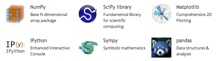
The IPython notebook is part of the IPython project. The IPython project is one of the packacges making up the python scientific stack called SciPi. SciPy (pronounced “Sigh Pie”) is a Python-based ecosystem of open-source software for mathematics, science, and engineering. In particular, these are some of the core packages:

SciPy

Quick IPython introdution¶

IPython provides a rich architecture for interactive computing with:

Powerful interactive shells (terminal and Qt-based).
A browser-based notebook with support for code, text, mathematical expressions, inline plots and other rich media.
Support for interactive data visualization and use of GUI toolkits.
Flexible, embeddable interpreters to load into your own projects.
Easy to use, high performance tools for parallel computing.

The main reasons I have been using it includes:

A superior shell
Plotting is possible in the QT console or the Notebook
the magic functions makes life easier (magics gets called with a %, use %-tab to see them all)
I also use it as a replacement shell for Windows Shell or Terminal
Code Completion
GNU Readline based editing and command history

Some helpfull commands¶

The four most helpful commands, as well as their brief description, is shown to you in a banner, every time you start IPython:

`command`	`description`
?	Introduction and overview of IPython's features.
%quickref	Quick reference.
help	Python's own help system.
object?	Details about 'object', use 'object??' for extra details.

Some imports and settings¶

The following code cells make sure that plotting is enabled and also loads a customised matplotlib confirguration file that spices up the inline plots. The custom matplotlib file has been taken from the Bayesian Methods for Hackers Project

In [3]:

# makes sure inline plotting is enabled
%pylab --no-import-all inline 

Populating the interactive namespace from numpy and matplotlib

In [4]:

#loads a customer marplotlib configuration file
def CustomPlot():
    import json
    s = json.load( open("static/matplotlibrc.json") )
    matplotlib.rcParams.update(s)
    figsize(18, 6) 

Changing the notebook layout¶

The code cell below is an example of how you should not be chaning the layout and css of the notebook. From IPython V1.00 it is possible to include custom css by creating IPython profiles. Since this file needs to be distributable I have opted for the hack below as used by the Bayesian Methods for Hackers Team

In [3]:

from IPython.core.display import HTML
def css_styling():
    styles = open("static/custom.css", "r").read()
    return HTML(styles)
css_styling()

Out[3]:

Notebook basics¶

The IPython Notebook is a web-based interactive computational environment where you can combine code execution, text, mathematics, plots and rich media into a single document.

Code Completion
Help
Docstrings
Markdown cells
Running a Code cell (Shift+Enter)
Setting a cell to be included in the presentation

Run the contents of a cell¶

SHIFT+ENTER will run the contents of a cell and move to the next one
CTRL+ENTER run the cell in place and don't move to the next cell. (best for presenting)
CTRL-m h show keyboard shorcuts

In [4]:

# press shift-enter to run code
print "Hallo Pycon"

Hallo Pycon

Save the notebook¶

CTRL-S will save the notebook

Lets get some help¶

The %quickref commmand can be used to obtain a bit more information

In [5]:

#IPython -- An enhanced Interactive Python - Quick Reference Card
%quickref  # now press shift-ender

Code completion and introspection¶

The cell below defines a function with a bit of a long name. By using the ? command the docstring can we viewed. ?? will open up the source code. The autocomplete function is also demostrated, and for fun the function is called and the output displayed

In [6]:

# lets degine a function with a long name.
def long_silly_dummy_name(a, b):
    """
    This is the docstring for dummy. 
    It takes two arguments a and b
    It returns the sum of a and b
    No error checking is done!
    """
    return a+b

In [7]:

# lets get the docstring or some help
long_silly_dummy_name?

In [ ]:

long_silly_dummy_name??

In [ ]:

#press tab to autocplete
long_si

In [8]:

# press shift-enter to run
long_silly_dummy_name(5,6)

Out[8]:

Setting up the notebook to enable a slideshow view¶

You need to activate the Cell Toolbar in the Toolbar above. Here you can set if this cell should be compiled as a slide or not. The options are given below:

slide
sub slide
fragment
skip
notes

Using markdown¶

You can set the contents type of a cell in the toolbar above. When Markdown is selected you can enter markdown in a cell and it's contents will be rendered as HTML. The markdown syntax can by found here

This is heading 1¶

This is heading 2¶

This is heading 5¶

Beautiful is better than ugly.

Explicit is better than implicit.
Simple is better than complex.
Complex is better than complicated.

Notebook magics¶

IPython has a set of predefined ‘magic functions’ that you can call with a command line style syntax. There are two kinds of magics, line-oriented and cell-oriented. Line magics are prefixed with the % character and work much like OS command-line calls: they get as an argument the rest of the line, where arguments are passed without parentheses or quotes. Cell magics are prefixed with a double %%, and they are functions that get as an argument not only the rest of the line, but also the lines below it in a separate argument.

Timeit magic¶

The timeit magic can be used to evaluate the average time your loop or piece of code is taking to complete it's run.

In [16]:

%%timeit 
x = 0   # setup
for i in range(100000):    #lets use range here
    x = x + i**2

100 loops, best of 3: 12.2 ms per loop

In [17]:

%%timeit 
x = 0   # setup
for i in xrange(100000):   #replace range with slightly improved xrange
    x += i**2

100 loops, best of 3: 10.7 ms per loop

Know when the kernel is busy¶

Have a look at the top right hand side of the notebook and run the code cell above again. This shows that the kernel is busy running the current cell.

User input¶

In the snippet below it the raw_input() function is used to read some user input to a variable raw and printed to stdout.

In [18]:

from IPython.display import HTML

raw = raw_input("enter your input here >>> ")

print "Hallo, ",raw

enter your input here >>> World!
Hallo,  World!

How to link to the filesystem¶

In [11]:

from IPython.display import FileLink, FileLinks
FileLinks('.', notebook_display_formatter=True)

Out[11]:

./
  .DS_Store
  builddocs.ipy
  calling_r_example.ipynb
  calling_ruby_example.ipynb
  pycon13_ipython.ipynb
  README.md
./.ipynb_checkpoints/
  calling_r_example-checkpoint.ipynb
  calling_ruby_example-checkpoint.ipynb
  pycon13_ipython-checkpoint.ipynb
./data/
  CapeTown_2009_Temperatures.csv
  READEME.md
./output/
  .DS_Store
  pycon13_ipython.html
  pycon13_ipython.slides.html
  pycon13_ipython_complete.pdf
  pycon13_ipython_pdf.pdf
./static/
  .DS_Store
  custom.css
  frontpage.docx
  frontpage.pdf
  ip.png
  ip2.png
  matplotlibrc.json
  python-vs-java.jpg
  scistack.png

Running shell commands¶

I now use ipython as my default shell scripting language. lets put the contents of the current directory into a list. by using the ! before a command indicates that you want to run a system command.

In [20]:

filelist = !ls                     #read the current directory into variable
for x,i in enumerate(filelist):
    print '#',x, '--->', i

# 0 ---> README.md
# 1 ---> builddocs.ipy
# 2 ---> calling_r_example.ipynb
# 3 ---> calling_ruby_example.ipynb
# 4 ---> data
# 5 ---> output
# 6 ---> pycon13_ipython.ipynb
# 7 ---> static

Embedding Images¶

Image released under CC BY-NC-ND 2.5 IN) by Rhul Singh

In [21]:

from IPython.display import Image
Image('static/python-vs-java.jpg')

Out[21]:

Adding YouYube videos¶

I am making the video small as it does not embed into the final output pdf.

In [22]:

from IPython.display import YouTubeVideo
YouTubeVideo('iwVvqwLDsJo', width=200, height=200)

Out[22]:

Plotting with Matplotlib¶

matplotlib is a python 2D plotting library which produces publication quality figures in a variety of hardcopy formats and interactive environments across platforms. matplotlib can be used in python scripts, the python and ipython shell, web application servers, and six graphical user interface toolkits.

In [23]:

from matplotlib.pylab import xkcd
#xkcd()
CustomPlot()
from numpy import *

#generate some data
n = array([0,1,2,3,4,5])
xx = np.linspace(-0.75, 1., 100)
x = linspace(0, 5, 10)
y = x ** 2

fig, axes = plt.subplots(1, 4, figsize=(12,3))

axes[0].scatter(xx, xx + 0.25*randn(len(xx)))
axes[0].set_title('scatter')
axes[1].step(n, n**2, lw=2)
axes[1].set_title('step')
axes[2].bar(n, n**2, align="center", width=0.5, alpha=0.5)
axes[2].set_title('bar')
axes[3].fill_between(x, x**2, x**3, color="green", alpha=0.5);
axes[3].set_title('fill')

for i in range(4):
    axes[i].set_xlabel('x')
axes[0].set_ylabel('y')
show()

Combined plots¶

In [24]:

CustomPlot()
font_size = 20
figsize(11.5, 6) 
fig, ax = plt.subplots()

ax.plot(xx, xx**2, xx, xx**3)
ax.set_title(r"Combined Plot $y=x^2$ vs. $y=x^3$", fontsize = font_size)
ax.set_xlabel(r'$x$', fontsize = font_size)
ax.set_ylabel(r'$y$', fontsize = font_size)
fig.tight_layout()
# inset
inset_ax = fig.add_axes([0.29, 0.45, 0.35, 0.35]) # X, Y, width, height
inset_ax.plot(xx, xx**2, xx, xx**3)
inset_ax.set_title(r'zoom $x=0$',fontsize=font_size)
# set axis range
inset_ax.set_xlim(-.2, .2)
inset_ax.set_ylim(-.005, .01)
# set axis tick locations
inset_ax.set_yticks([0, 0.005, 0.01])
inset_ax.set_xticks([-0.1,0,.1]);
show()

Adding text to a plot¶

In [25]:

CustomPlot()
figsize(11.5, 6) 
font_size = 20
fig, ax = plt.subplots()
ax.plot(xx, xx**2, xx, xx**3)
ax.set_xlabel(r'$x$', fontsize = font_size)
ax.set_ylabel(r'$y$', fontsize = font_size)
ax.set_title(r"Adding Text $y=x^2$ vs. $y=x^3$", fontsize = font_size)
ax.text(0.15, 0.2, r"$y=x^2$", fontsize=font_size, color="blue")
ax.text(0.65, 0.1, r"$y=x^3$", fontsize=font_size, color="green");

xkcd style plotting¶

matplolib v1.3 now includes a setting to make plots resemple xkcd styles.

In [26]:

from matplotlib import pyplot as plt
import numpy as np

plt.xkcd()

fig = plt.figure()
ax = fig.add_subplot(1, 1, 1)
ax.spines['right'].set_color('none')
ax.spines['top'].set_color('none')
plt.xticks([])
plt.yticks([])
ax.set_ylim([-30, 10])

data = np.ones(100)
data[70:] -= np.arange(30)

plt.annotate(
    'THE DAY I REALIZED\nI COULD COOK BACON\nWHENEVER I WANTED',
    xy=(70, 1), arrowprops=dict(arrowstyle='->'), xytext=(15, -10))

plt.plot(data)

plt.xlabel('time')
plt.ylabel('my overall health')

fig = plt.figure()
ax = fig.add_subplot(1, 1, 1)
ax.bar([-0.125, 1.0-0.125], [0, 100], 0.25)
ax.spines['right'].set_color('none')
ax.spines['top'].set_color('none')
ax.xaxis.set_ticks_position('bottom')
ax.set_xticks([0, 1])
ax.set_xlim([-0.5, 1.5])
ax.set_ylim([0, 110])
ax.set_xticklabels(['CONFIRMED BY\nEXPERIMENT', 'REFUTED BY\nEXPERIMENT'])
plt.yticks([])

plt.title("CLAIMS OF SUPERNATURAL POWERS")

plt.show()

Symbolic math using SymPy¶

SymPy is a Python library for symbolic mathematics. It aims to become a full-featured computer algebra system (CAS) while keeping the code as simple as possible in order to be comprehensible and easily extensible. SymPy is written entirely in Python and does not require any external libraries.

In [27]:

from sympy import *
init_printing(use_latex=True)
x = Symbol('x')
y = Symbol('y')
series(exp(x), x, 1, 5)

Out[27]:

$$e + e x + \frac{1}{2} e x^{2} + \frac{1}{6} e x^{3} + \frac{1}{24} e x^{4} + \mathcal{O}\left(x^{5}\right)$$

In [28]:

eq = ((x+y)**2 * (x+1))
eq

Out[28]:

$$\left(x + 1\right) \left(x + y\right)^{2}$$

In [29]:

expand(eq)

Out[29]:

$$x^{3} + 2 x^{2} y + x^{2} + x y^{2} + 2 x y + y^{2}$$

In [30]:

a = 1/x + (x*sin(x) - 1)/x
a

Out[30]:

$$\frac{x \sin{\left (x \right )} -1}{x} + \frac{1}{x}$$

In [31]:

simplify(a)

Out[31]:

$$\sin{\left (x \right )}$$

Data analysis using the Pandas library¶

pandas is a Python package providing fast, flexible, and expressive data structures designed to make working with “relational” or “labeled” data both easy and intuitive

The two primary data structures of pandas, Series (1-dimensional) and DataFrame (2-dimensional), handle the vast majority of typical use cases in finance, statistics, social science, and many areas of engineering.

For R users, DataFrame provides everything that R’s data.frame provides and much more. pandas is built on top of NumPy and is intended to integrate well within a scientific computing environment with many other 3rd party libraries.

In [32]:

from pandas import DataFrame, read_csv

Cape_Weather = DataFrame( read_csv('data/CapeTown_2009_Temperatures.csv' ))
Cape_Weather.head()

Out[32]:

	high	low	radiation
0	25	16	29.0
1	23	15	25.7
2	25	15	21.5
3	26	16	15.2
4	26	17	10.8

In [33]:

CustomPlot()
figsize(11.5, 6)
font_size = 20
title('Cape Town temparature(2009)',fontsize = font_size)
xlabel('Day number',fontsize = font_size)
ylabel(r'Temperature [$^\circ C$] ',fontsize = font_size)
Cape_Weather.high.plot()
Cape_Weather.low.plot()
show()