Worksheet 8 - Regression
Lecture and Tutorial Learning Goals:
After completing this week's lecture and tutorial work, you will be able to:
- Recognize situations where a simple regression analysis would be appropriate for making predictions.
- Explain the k-nearest neighbour ($k$-nn) regression algorithm and describe how it differs from $k$-nn classification.
- Interpret the output of a $k$-nn regression.
- In a dataset with two variables, perform k-nearest neighbour regression in R using
tidymodelsto predict the values for a test dataset. - Using R, execute cross-validation in R to choose the number of neighbours.
- Using R, evaluate $k$-nn regression prediction accuracy using a test data set and an appropriate metric (e.g., root mean square prediction error, RMSPE).
- In the context of $k$-nn regression, compare and contrast goodness of fit and prediction properties (namely RMSE vs RMSPE).
- Describe advantages and disadvantages of the $k$-nearest neighbour regression approach.
This worksheet covers parts of the Regression I chapter of the online textbook. You should read this chapter before attempting the worksheet.
### Run this cell before continuing.
library(tidyverse)
library(repr)
library(tidymodels)
options(repr.matrix.max.rows = 6)
source("tests.R")
source('cleanup.R')
Question 0.0 Multiple Choice:
{points: 1}
To predict a value of $Y$ for a new observation using $k$-nn regression, we identify the $k$-nearest neighbours and then:
A. Assign it the median of the $k$-nearest neighbours as the predicted value
B. Assign it the mean of the $k$-nearest neighbours as the predicted value
C. Assign it the mode of the $k$-nearest neighbours as the predicted value
D. Assign it the majority vote of the $k$-nearest neighbours as the predicted value
Save the letter of the answer you think is correct to a variable named answer0.0. Make sure your answer is an uppercase letter and is surrounded by quotation marks (e.g. "F").
# your code here
fail() # No Answer - remove if you provide an answer
answer0.0
test_0.0()
Question 0.1 Multiple Choice:
{points: 1}
Of those shown below, which is the correct formula for RMSPE?
A. $RMSPE = \sqrt{\frac{\frac{1}{n}\sum\limits_{i=1}^{n}(y_i - \hat{y_i})^2}{1 - n}}$
B. $RMSPE = \sqrt{\frac{1}{n - 1}\sum\limits_{i=1}^{n}(y_i - \hat{y_i})^2}$
C. $RMSPE = \sqrt{\frac{1}{n}\sum\limits_{i=1}^{n}(y_i - \hat{y_i})^2}$
D. $RMSPE = \sqrt{\frac{1}{n}\sum\limits_{i=1}^{n}(y_i - \hat{y_i})}$
Save the letter of the answer you think is correct to a variable named answer0.1. Make sure you put quotations around the letter and pay attention to case.
# your code here
fail() # No Answer - remove if you provide an answer
answer0.1
test_0.1()
Question 0.2
{points: 1}
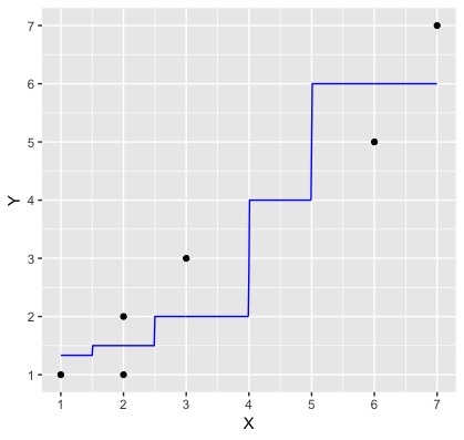
The plot below is a very simple k-nn regression example, where the black dots are the data observations and the blue line is the predictions from a $k$-nn regression model created from this data where $k=2$.
Using the formula for RMSE (given in the reading), and the graph below, by hand (pen and paper or use R as a calculator) calculate RMSE for this model. Use one decimal place of precision when inputting the heights of the black dots and blue line. Save your answer to a variable named answer0.2
Note: The predicted value when x = 1 is 1.3 (it's a bit hard to tell from the figure!)
# your code here
fail() # No Answer - remove if you provide an answer
answer0.2
test_0.2()
RMSPE Definition
Question 0.3 Multiple Choice:
{points: 1}
What does RMSPE stand for?
A. root mean squared prediction error
B. root mean squared percentage error
C. root mean squared performance error
D. root mean squared preference error
Save the letter of the answer you think is correct to a variable named answer0.3. Make sure you put quotations around the letter and pay attention to case.
# your code here
fail() # No Answer - remove if you provide an answer
answer0.3
test_0.3()
Marathon Training
Source: https://media.giphy.com/media/nUN6InE2CodRm/giphy.gif
What predicts which athletes will perform better than others? Specifically, we are interested in marathon runners, and looking at how the maximum distance ran per week (in miles) during race training predicts the time it takes a runner to finish the race? For this, we will be looking at the marathon.csv file in the data/ folder.
Question 1.0
{points: 1}
Load the data and assign it to an object called marathon.
# your code here
fail() # No Answer - remove if you provide an answer
marathon
test_1.0()
Question 2.0
{points: 1}
We want to predict race time (in hours) (time_hrs) given a particular value of maximum distance ran per week (in miles) during race training (max). Let's take a subset of size 50 individuals of our marathon data and assign it to an object called marathon_50. With this subset, plot a scatterplot to assess the relationship between these two variables. Put time_hrs on the y-axis and max on the x-axis. Assign this plot to an object called answer2. Discuss, with a classmate, the relationship between race time and maximum distance ran per week during training based on the scatterplot you create below.
Hint: To take a subset of your data you can use the sample_n() function
options(repr.plot.width = 8, repr.plot.height = 7)

set.seed(2000) ### DO NOT CHANGE

#... <- ... |>
#    sample_n(...)

# your code here
fail() # No Answer - remove if you provide an answer
answer2
test_2.0()
Question 3.0
{points: 1}
Suppose we want to predict the race time for someone who ran a maximum distance of 100 miles per week during training. In the plot below we can see that no one has run a maximum distance of 100 miles per week. But, if we are interested in prediction, how can we predict with this data? We can use $k$-nn regression! To do this we get the $Y$ values (target/response variable) of the nearest $k$ values and then take their average and use that as the prediction.
For this question predict the race time based on the 4 closest neighbors to the 100 miles per week during training.
Fill in the scaffolding below and assign your answer to an object named answer3.
# run this cell to see a visualization of the 4 nearest neighbours
options(repr.plot.height = 6, repr.plot.width = 7)
marathon_50 |>
    ggplot(aes(x = max, y = time_hrs)) +
        geom_point(color = 'dodgerblue', alpha = 0.4) +
        geom_vline(xintercept = 100, linetype = "dotted") +
        xlab("Maximum Distance Ran per \n Week During Training (mi)") +
        ylab("Race Time (hours)") +
        geom_segment(aes(x = 100, y = 2.56, xend = 107, yend = 2.56), col = "orange") +
        geom_segment(aes(x = 100, y = 2.65, xend = 90, yend = 2.65), col = "orange") +
        geom_segment(aes(x = 100, y = 2.99, xend = 86, yend = 2.99), col = "orange") +
        geom_segment(aes(x = 100, y = 3.05, xend = 82, yend = 3.05), col = "orange") +
        theme(text = element_text(size = 20))
#... <- ... |>
#  mutate(diff = abs(100 - ...)) |>
#  ...(diff, ...) |>
#  summarise(predicted = ...(...)) |>
#  pull()

# your code here
fail() # No Answer - remove if you provide an answer
answer3
test_3.0()
Question 4.0
{points: 1}
For this question, let's instead predict the race time based on the 2 closest neighbors to the 100 miles per week during training.
Assign your answer to an object named answer4.
# your code here
fail() # No Answer - remove if you provide an answer
answer4
test_4.0()
Question 5.0 Multiple Choice:
{points: 1}
So far you have calculated the $k$ nearest neighbors predictions manually based on $k$'s we have told you to use. However, last week we learned how to use a better method to choose the best $k$ for classification.
Based on what you learned last week and what you have learned about $k$-nn regression so far this week, which method would you use to choose the $k$ (in the situation where we don't tell you which $k$ to use)?
- A) Choose the $k$ that excludes most outliers
- B) Choose the $k$ with the lowest training error
- C) Choose the $k$ with the lowest cross-validation error
- D) Choose the $k$ that includes the most data points
- E) Choose the $k$ with the lowest testing error
Assign your answer to an object called answer5. Make sure your answer is an uppercase letter and is surrounded by quotation marks (e.g. "F").
# your code here
fail() # No Answer - remove if you provide an answer
answer5
test_5.0()
Question 6.0
{points: 1}
We have just seen how to perform k-nn regression manually, now we will apply it to the whole dataset using the tidymodels package. To do so, we will first need to create the training and testing datasets. Split the data using 75% of the marathon data as your training set and set time_hrs as the strata argument. Store this data into an object called marathon_split.
Then, use the appropriate training and testing functions to create your training set which you will call marathon_training and your testing set which you will call marathon_testing. Remember we won't touch the test dataset until the end.
set.seed(2000) ### DO NOT CHANGE

#... <- initial_split(..., prop = ..., strata = ...)
#... <- training(...)
#... <- testing(...)


# your code here
fail() # No Answer - remove if you provide an answer
test_6.0()
Question 7.0
{points: 1}
Next, we’ll use cross-validation on our training data to choose $k$. In $k$-nn classification, we used accuracy to see how well our predictions matched the true labels. In the context of $k$-nn regression, we will use RMPSE instead. Interpreting the RMPSE value can be tricky but generally speaking, if the prediction values are very close to the true values, the RMSPE will be small. Conversely, if the prediction values are not very close to the true values, the RMSPE will be quite large.
Let's perform a cross-validation and choose the optimal $k$. First, create a model specification for $k$-nn. We are still using the $k$-nearest neighbours algorithm, and so we will still use the same package for the model engine as we did in classification ("kknn"). As usual, specify that we want to use the straight-line distance. However, since this will be a regression problem, we will use set_mode("regression") in the model specification. Store your model specification in an object called marathon_spec.
Moreover, create a recipe to preprocess our data. Store your recipe in an object called marathon_recipe. The recipe should specify that the response variable is race time (hrs) and the predictor is maximum distance ran per week during training.
set.seed(1234) #DO NOT REMOVE

#... <- nearest_neighbor(weight_func = ..., neighbors = ...) |>
#       set_engine(...) |>
#       set_mode(...)

#... <- recipe(... ~ ..., data = ...) |>
#       step_scale(...) |>
#       step_center(...)
#

# your code here
fail() # No Answer - remove if you provide an answer
marathon_recipe
test_7.0()
Question 7.1
{points: 1}
Now, create the splits for cross-validation with 5 folds using the vfold_cv function. Store your answer in an object called marathon_vfold. Make sure to set the strata argument.
Then, use the workflow function to combine your model specification and recipe. Store your answer in an object called marathon_workflow.
set.seed(1234) # DO NOT REMOVE

# your code here
fail() # No Answer - remove if you provide an answer
marathon_workflow
test_7.1()
Question 8.0
{points: 1}
If you haven't noticed by now, the major difference compared to other workflows from Chapters 6 and 7 is that we are running a regression rather than a classification. Specifying regression in the set_mode function essentially tells tidymodels that we need to use different metrics (RMPSE rather than accuracy) for tuning and evaluation.
Now, let's use the RMSPE to find the best setting for $k$ from our workflow. Let's test the values $k = 1, 11, 21, 31, ..., 81$.
First, create a tibble with a column called neighbors that contains the sequence of values. Remember that you should use the seq function to create the range of $k$s that goes from 1 to 81 by jumps of 10. Assign that tibble to an object called gridvals.
Next, tune your workflow such that it tests all the values in gridvals and resamples using your cross-validation data set. Finally, collect the statistics from your model. Assign your answer to an object called marathon_results.
set.seed(2019) # DO NOT CHANGE
# your code here
fail() # No Answer - remove if you provide an answer
marathon_results
test_8.0()
Question 8.1
{points: 1}
Great! Now find the minimum RMSPE along with it's associated metrics such as the mean and standard error, to help us find the number of neighbors that will serve as our best $k$ value. Your answer should simply be a tibble with one row. Assign your answer to an object called marathon_min.
set.seed(2020) # DO NOT REMOVE

#... <- marathon_results |>
#    filter(.metric == ...) |>
#    slice_min(..., ...)

# your code here
fail() # No Answer - remove if you provide an answer
marathon_min
test_8.1()
Question 8.2
{points: 1}
To assess how well our model might do at predicting on unseen data, we will assess its RMSPE on the test data. To do this, we will first re-train our $k$-nn regression model on the entire training data set, using the $K$ value we obtained from Question 8.1.
To start, pull the best neighbors value from marathon_min and store it an object called k_min.
Following that, we will repeat the workflow analysis again but with a brand new model specification with k_min. Remember, we are doing a regression analysis, so please select the appropriate mode. Store your new model specification in an object called marathon_best_spec and your new workflow analysis in an object called marathon_best_fit. You can reuse this marathon_recipe for this workflow, as we do not need to change it for this task.
Then, we will use the predict function to make predictions on the test data, and use the metrics function again to compute a summary of the regression's quality. Store your answer in an object called marathon_summary.
set.seed(1234) # DO NOT REMOVE

#... <- marathon_min |>
#          pull(...)

#... <- nearest_neighbor(weight_func = ..., neighbors = ...) |>
#          set_engine(...) |>
#          set_mode(...)

#... <- workflow() |>
#          add_recipe(...) |>
#          add_model(...) |>
#          fit(data = ...)

#... <- marathon_best_fit |>
#           predict(...) |>
#           bind_cols(...) |>
#           metrics(truth = ..., estimate = ...)

# your code here
fail() # No Answer - remove if you provide an answer
marathon_summary
test_8.2()
What does this RMSPE score mean? RMSPE is measured in the units of the target/response variable, so it can sometimes be a bit hard to interpret. But in this case, we know that a typical marathon race time is somewhere between 3 - 5 hours. So this model allows us to predict a runner's race time up to about +/-0.6 of an hour, or +/- 36 minutes. This is not fantastic, but not terrible either. We can certainly use the model to determine roughly whether an athlete will have a bad, good, or excellent race time, but probably cannot reliably distinguish between athletes of a similar caliber.
For now, let’s consider this approach to thinking about RMSPE from our testing data set: as long as its not significantly worse than the cross-validation RMSPE of our best model (Question 8.1), then we can say that we’re not doing too much worse on the test data than we did on the training data. In future courses on statistical/machine learning, you will learn more about how to interpret RMSPE from testing data and other ways to assess models.
Question 8.3 True or False:
{points: 1}
The RMPSE from our testing data set is much worse than the cross-validation RMPSE of our best model.
Assign your answer to an object named answer8.3. Make sure your answer is in lowercase and is surrounded by quotation marks (e.g. "true" or "false").
# your code here
fail() # No Answer - remove if you provide an answer
test_8.3()
Question 9.0
{points: 1}
Let's visualize what the relationship between max and time_hrs looks like with our best $k$ value to ultimately explore how the $k$ value affects $k$-nn regression.
To do so, use the predict function on the workflow analysis that utilizes the best $k$ value (marathon_best_fit) to create predictions for the marathon_training data. Then, add the column of predictions to the marathon_training data frame using bind_cols. Name the resulting data frame marathon_preds.
Next, create a scatterplot with the maximum distance ran per week against the marathon time from marathon_preds. Assign your plot to an object called marathon_plot. Plot the predictions as a blue line over the data points. Remember the fundamentals of effective visualizations such as having a title and human-readable axes.
Note: use geom_point before geom_line when creating the plot to ensure tests pass!
set.seed(2019) # DO NOT CHANGE

options(repr.plot.width = 7, repr.plot.height = 7)

# your code here
fail() # No Answer - remove if you provide an answer
marathon_plot
test_9.0()
source('cleanup.R')