Visualizing Image Data
This notebook will demonstrate how to load and visualize astronomical images in the pywwt viewer.
Step 1: Starting up pywwt
The first thing to do is to open up a pywwt window in this notebook session. As is generally the case, we have to start with some Python imports:
from pywwt.jupyter import WWTJupyterWidget
We'll also set up a utility function to help us load data files stored alongside this notebook:
def datapath(*args):
    from os.path import join
    return join('data', *args)
Next, create a widget and display it inline. (That's why the final line is a bare wwt.)
wwt = WWTJupyterWidget()
wwt
If everything is working correctly, the above command should create a pywwt viewer that looks mostly like a black box. If you’re using the JupyterLab environment rather than a plain Jupyter notebook, it is strongly recommended that you move the viewer to its own window pane so that you can have your code and viz side-by-side:
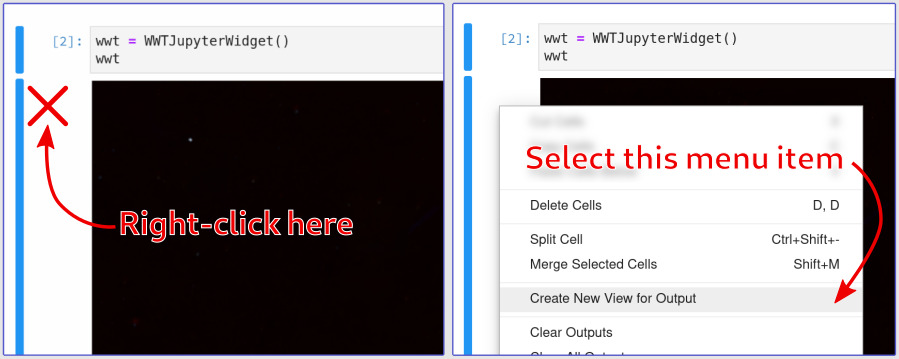
If you don't get a menu or the menu doesn’t look like the one pictured, you are probably not using JupyterLab and will have to move the viewer cell down as you work your way through the notebook. See the First Steps notebook for more information and troubleshooting tips if you don’t get a viewer at all.
Step 2: Visualizing a Local FITS file
We'll start by visualizing a WISE 12µm image towards the Westerhout 5 star forming region and taking a look at some of the advanced visualization options.
Images, like data tables, are represented in WWT as "layers" that can be added to the view. With a standard FITS file, all you need to do is provide a pathname:
layer = wwt.layers.add_image_layer(datapath('w5.fits'))
The viewer will automatically center and zoom to the image you've loaded. You may get a warning from the reproject module; this can safely be ignored.
"Printing" the following variable will create a set of widgets that let you adjust how the data are visualized:
layer.controls
The image color scaling is controlled by the sliders in the "Fine min/max" row; the "Coarse min/max" boxes control the bounds that are placed on the range of those sliders.
You should try sliding the image opacity back and forth to check the agreement between the morphology of the W5 image and the WWT all-sky map.
All of the parameters that are controlled by the widgets above can be manipulated programmatically as well. Let's set a bunch of them at once:
layer.cmap = 'plasma'
layer.vmin = 400
layer.vmax = 1000
layer.stretch = 'sqrt'
layer.opacity = 0.9
Note that the settings in the widgets adjusted automatically to match what you entered. Fancy!
After you're done playing around, let's reset the WWT widget:
wwt.reset()
Step 3: Loading data from remote sources
Because pywwt is a Python module, not a standalone application, it gains a lot of power by being able to integrate with other components of the modern, Web-oriented astronomical software ecosystem.
For instance, it is easy to use the Python module astroquery to load in data directly from archive queries, without the requirement to save any files locally. Let's fetch 2MASS Ks-band images of the field of supernova 2011fe. This might take a little while since the Python kernel needs to download the data from MAST.
Temporarily using SDSS-u instead of 2MASS-Ks since SkyView's 2MASS service is currently down. (2020 Nov)
from astroquery.skyview import SkyView

img_list = SkyView.get_images(
    position='SN 2011FE',
    survey='SDSSu',
    pixels=700  # you can adjust the size if you want
)
assert len(img_list) == 1  # there's only one matching item in this example
twomass_img = img_list[0]
twomass_img.info()
Once the FITS data are available, we can display them in pywwt using the same command as before:
twomass_layer = wwt.layers.add_image_layer(twomass_img)
Once again you should see the view automatically center on your image. Let's adjust the background imagery to be more relevant:
wwt.background = wwt.imagery.ir.twomass
wwt.foreground_opacity = 0
pywwt provides interactive controls to let you adjust the parameters of the contextual imagery that's being shown. Try choosing different sets of all-sky imagery and adjusting the blend between them:
wwt.layer_controls
Here are some settings that we like:
wwt.background = wwt.imagery.visible.sdss
wwt.foreground = wwt.imagery.gamma.fermi
wwt.foreground_opacity = .5
Now we'll load up another image of the same field that came from Swift, this time stored as a local file as in the previous step:
swift_layer = wwt.layers.add_image_layer(datapath('m101_swiftx.fits'))
Create controls to adjust all of the visualization parameters. If you want to go wild, you can overlay data from four different wavelengths in this one view!
wwt.layer_controls
twomass_layer.controls
swift_layer.controls
Next Steps
To learn how to display data tables along with your imagery, start with the NASA Exoplanet Archive tutorial