4 Python Static¶

파이썬을 활용한 금융분석

## **1 기술통계 계산과 요약** 기본적인 수학/ 통계 메소드(함수)

### **01 기술통계** 엑셀의 함수를 더 쉽고, 빠르게 적용 가능하다

In [1]:

import pandas as pd
import numpy as np
data = np.arange(20).reshape((4,5))
data

Out[1]:

array([[ 0,  1,  2,  3,  4],
       [ 5,  6,  7,  8,  9],
       [10, 11, 12, 13, 14],
       [15, 16, 17, 18, 19]])

In [2]:

df = pd.DataFrame(data, 
                  index   = ['three', 'one', 'two', 'five'], 
                  columns = [ 'd', 'e', 'f', 'a', 'g'])
df

Out[2]:

	d	e	f	a	g
three	0	1	2	3	4
one	5	6	7	8	9
two	10	11	12	13	14
five	15	16	17	18	19

In [3]:

df.quantile(q=0.05)

Out[3]:

d    0.75
e    1.75
f    2.75
a    3.75
g    4.75
Name: 0.05, dtype: float64

In [4]:

df.sum( ) 

Out[4]:

d    30
e    34
f    38
a    42
g    46
dtype: int64

In [5]:

df.sum( axis = 1 )

Out[5]:

three    10
one      35
two      60
five     85
dtype: int64

In [6]:

df.mean( axis=0 , skipna = False )

Out[6]:

d     7.5
e     8.5
f     9.5
a    10.5
g    11.5
dtype: float64

In [7]:

df.count()

Out[7]:

d    4
e    4
f    4
a    4
g    4
dtype: int64

In [8]:

df.cumsum()

Out[8]:

	d	e	f	a	g
three	0	1	2	3	4
one	5	7	9	11	13
two	15	18	21	24	27
five	30	34	38	42	46

In [9]:

df.cumprod()

Out[9]:

	e	f	a	g
three	1	2	3	4
one	6	14	24	36
two	66	168	312	504
five	1056	2856	5616	9576

In [10]:

df.describe()

Out[10]:

	d	e	f	a	g
count	4.000000	4.000000	4.000000	4.000000	4.000000
mean	7.500000	8.500000	9.500000	10.500000	11.500000
std	6.454972	6.454972	6.454972	6.454972	6.454972
min	0.000000	1.000000	2.000000	3.000000	4.000000
25%	3.750000	4.750000	5.750000	6.750000	7.750000
50%	7.500000	8.500000	9.500000	10.500000	11.500000
75%	11.250000	12.250000	13.250000	14.250000	15.250000
max	15.000000	16.000000	17.000000	18.000000	19.000000

In [11]:

df.pct_change()

Out[11]:

	d	e	f	a	g
three	NaN	NaN	NaN	NaN	NaN
one	inf	5.000000	2.500000	1.666667	1.250000
two	1.000000	0.833333	0.714286	0.625000	0.555556
five	0.500000	0.454545	0.416667	0.384615	0.357143

In [12]:

%matplotlib inline
df.pct_change().plot(kind='line')

Out[12]:

<matplotlib.axes._subplots.AxesSubplot at 0x7f6f20aa55f8>

## **2 결측치(np.Nan) 제어하기**
### **01 결측치(np.Nan) 찾기**

In [13]:

data  = pd.Series([20000,1200,2500],  index = ['매출액', '영업이익' ,'대손충당금'])
data2 = pd.Series([34000,120,360],    index = ['매출액', '당기순이익','대손충당금'])
df = pd.DataFrame( {'2017Y4Q': data, '2018Y1Q': data2 },
                 index = ['매출액', '영업이익', '당기순이익', '대손충당금']) 
df

Out[13]:

	2017Y4Q	2018Y1Q
매출액	20000.0	34000.0
영업이익	1200.0	NaN
당기순이익	NaN	120.0
대손충당금	2500.0	360.0

In [14]:

df.dropna()

Out[14]:

	2017Y4Q	2018Y1Q
매출액	20000.0	34000.0
대손충당금	2500.0	360.0

In [15]:

print(df.isnull().sum())
print('\n2017Y4Q', df[df['2017Y4Q'].isnull()].index)
print('\n2018Y1Q', df[df['2018Y1Q'].isnull()].index)

2017Y4Q    1
2018Y1Q    1
dtype: int64

2017Y4Q Index(['당기순이익'], dtype='object')

2018Y1Q Index(['영업이익'], dtype='object')

### **02 결측치(np.Nan) 채우기**

In [16]:

df.fillna(0)

Out[16]:

	2017Y4Q	2018Y1Q
매출액	20000.0	34000.0
영업이익	1200.0	0.0
당기순이익	0.0	120.0
대손충당금	2500.0	360.0

In [17]:

df.fillna(method='ffill',  limit=2)  

Out[17]:

	2017Y4Q	2018Y1Q
매출액	20000.0	34000.0
영업이익	1200.0	34000.0
당기순이익	1200.0	120.0
대손충당금	2500.0	360.0

In [18]:

df.fillna(method='bfill')

Out[18]:

	2017Y4Q	2018Y1Q
매출액	20000.0	34000.0
영업이익	1200.0	120.0
당기순이익	2500.0	120.0
대손충당금	2500.0	360.0

In [19]:

df.fillna(df.mean())

Out[19]:

	2017Y4Q	2018Y1Q
매출액	20000.0	34000.000000
영업이익	1200.0	11493.333333
당기순이익	7900.0	120.000000
대손충당금	2500.0	360.000000

In [20]:

df.fillna(df.mean()['2017Y4Q'])

Out[20]:

	2017Y4Q	2018Y1Q
매출액	20000.0	34000.0
영업이익	1200.0	7900.0
당기순이익	7900.0	120.0
대손충당금	2500.0	360.0

### **03 결측치(np.Nan) 보간법으로 대체하기**

In [21]:

import pandas as pd
import numpy as np
from pandas import DataFrame, Series
from datetime import datetime

datestrs   = ['12/1/2016', '12/03/2016', '12/04/2016', '12/10/2016']
dates      = pd.to_datetime(datestrs)
timeSeries = Series([1, np.nan, np.nan, 10], index=dates)
print(timeSeries.index)
timeSeries

DatetimeIndex(['2016-12-01', '2016-12-03', '2016-12-04', '2016-12-10'], dtype='datetime64[ns]', freq=None)

Out[21]:

2016-12-01     1.0
2016-12-03     NaN
2016-12-04     NaN
2016-12-10    10.0
dtype: float64

In [22]:

%matplotlib inline
timeSeries.interpolate().plot()
timeSeries.interpolate()

Out[22]:

2016-12-01     1.0
2016-12-03     4.0
2016-12-04     7.0
2016-12-10    10.0
dtype: float64

In [23]:

timeSeries.interpolate(method='time').plot()
timeSeries.interpolate(method='time')

Out[23]:

2016-12-01     1.0
2016-12-03     3.0
2016-12-04     4.0
2016-12-10    10.0
dtype: float64

In [24]:

timeSeries.interpolate(method='values').plot()
timeSeries.interpolate(method='values')

Out[24]:

2016-12-01     1.0
2016-12-03     3.0
2016-12-04     4.0
2016-12-10    10.0
dtype: float64

In [25]:

timeSeries.interpolate(method='values', limit=1)

Out[25]:

2016-12-01     1.0
2016-12-03     3.0
2016-12-04     NaN
2016-12-10    10.0
dtype: float64

In [26]:

timeSeries.interpolate(method='values', limit=1, limit_direction='backward')

Out[26]:

2016-12-01     1.0
2016-12-03     NaN
2016-12-04     4.0
2016-12-10    10.0
dtype: float64

3. Time Series¶

시계열 데이터 처리하기

### **01 DateTimeSeries** 시간 데이터 관리하기

In [27]:

from time import time
time()   

Out[27]:

1526350402.8931286

In [28]:

t0 = time()
for i in range(100_000_000):
    pass
int( time() - t0 )

Out[28]:

### **02 Date & Time** 날짜와 시간관리

In [29]:

from datetime import datetime
dt = datetime.now()
dt

Out[29]:

datetime.datetime(2018, 5, 15, 11, 13, 26, 108631)

In [30]:

print('year'     , dt.year, 
      '\nmonth'  , dt.month, 
      '\nday'    , dt.day, 
      '\nhour'   , dt.hour, 
      '\nminute' , dt.minute, 
      '\nsecond' , dt.second, 
      dt.microsecond)

year 2018 
month 5 
day 15 
hour 11 
minute 13 
second 26 108631

### **03 Time stamp & Date** 날짜와 시간관리 데이터 상호교환

In [31]:

datetime.fromtimestamp(0)

Out[31]:

datetime.datetime(1970, 1, 1, 9, 0)

In [32]:

now = time()
print(now)
datetime.fromtimestamp(now)

1526350406.1359463

Out[32]:

datetime.datetime(2018, 5, 15, 11, 13, 26, 135946)

In [33]:

date = datetime(2017, 10, 21, 16, 29, 0)
date

Out[33]:

datetime.datetime(2017, 10, 21, 16, 29)

In [34]:

date.strftime('%Y/%m/%d %H:%M:%S')

Out[34]:

'2017/10/21 16:29:00'

In [35]:

date.strftime('%Y/%m/%d')

Out[35]:

'2017/10/21'

In [36]:

date.strftime('%Y-%m-%d')

Out[36]:

'2017-10-21'

### **04 Datetime in Pandas** **Series.resample()** freq 옵션 [code](https://datascienceschool.net/view-notebook/8959673a97214e8fafdb159f254185e9/)

#### **1) pandas.date_range()**

In [37]:

pd.date_range('2017/01/01','2017/01/31')

Out[37]:

DatetimeIndex(['2017-01-01', '2017-01-02', '2017-01-03', '2017-01-04',
               '2017-01-05', '2017-01-06', '2017-01-07', '2017-01-08',
               '2017-01-09', '2017-01-10', '2017-01-11', '2017-01-12',
               '2017-01-13', '2017-01-14', '2017-01-15', '2017-01-16',
               '2017-01-17', '2017-01-18', '2017-01-19', '2017-01-20',
               '2017-01-21', '2017-01-22', '2017-01-23', '2017-01-24',
               '2017-01-25', '2017-01-26', '2017-01-27', '2017-01-28',
               '2017-01-29', '2017-01-30', '2017-01-31'],
              dtype='datetime64[ns]', freq='D')

In [38]:

pd.date_range('2017-07-01', periods=30)

Out[38]:

DatetimeIndex(['2017-07-01', '2017-07-02', '2017-07-03', '2017-07-04',
               '2017-07-05', '2017-07-06', '2017-07-07', '2017-07-08',
               '2017-07-09', '2017-07-10', '2017-07-11', '2017-07-12',
               '2017-07-13', '2017-07-14', '2017-07-15', '2017-07-16',
               '2017-07-17', '2017-07-18', '2017-07-19', '2017-07-20',
               '2017-07-21', '2017-07-22', '2017-07-23', '2017-07-24',
               '2017-07-25', '2017-07-26', '2017-07-27', '2017-07-28',
               '2017-07-29', '2017-07-30'],
              dtype='datetime64[ns]', freq='D')

In [39]:

pd.date_range(end = '2017-07-01', periods=30)

Out[39]:

DatetimeIndex(['2017-06-02', '2017-06-03', '2017-06-04', '2017-06-05',
               '2017-06-06', '2017-06-07', '2017-06-08', '2017-06-09',
               '2017-06-10', '2017-06-11', '2017-06-12', '2017-06-13',
               '2017-06-14', '2017-06-15', '2017-06-16', '2017-06-17',
               '2017-06-18', '2017-06-19', '2017-06-20', '2017-06-21',
               '2017-06-22', '2017-06-23', '2017-06-24', '2017-06-25',
               '2017-06-26', '2017-06-27', '2017-06-28', '2017-06-29',
               '2017-06-30', '2017-07-01'],
              dtype='datetime64[ns]', freq='D')

In [40]:

pd.date_range(end = '2017-07-01', periods=30, freq='B')  

Out[40]:

DatetimeIndex(['2017-05-22', '2017-05-23', '2017-05-24', '2017-05-25',
               '2017-05-26', '2017-05-29', '2017-05-30', '2017-05-31',
               '2017-06-01', '2017-06-02', '2017-06-05', '2017-06-06',
               '2017-06-07', '2017-06-08', '2017-06-09', '2017-06-12',
               '2017-06-13', '2017-06-14', '2017-06-15', '2017-06-16',
               '2017-06-19', '2017-06-20', '2017-06-21', '2017-06-22',
               '2017-06-23', '2017-06-26', '2017-06-27', '2017-06-28',
               '2017-06-29', '2017-06-30'],
              dtype='datetime64[ns]', freq='B')

In [41]:

pd.date_range(end = '2017-07-01', periods=30, freq='BM')  

Out[41]:

DatetimeIndex(['2015-01-30', '2015-02-27', '2015-03-31', '2015-04-30',
               '2015-05-29', '2015-06-30', '2015-07-31', '2015-08-31',
               '2015-09-30', '2015-10-30', '2015-11-30', '2015-12-31',
               '2016-01-29', '2016-02-29', '2016-03-31', '2016-04-29',
               '2016-05-31', '2016-06-30', '2016-07-29', '2016-08-31',
               '2016-09-30', '2016-10-31', '2016-11-30', '2016-12-30',
               '2017-01-31', '2017-02-28', '2017-03-31', '2017-04-28',
               '2017-05-31', '2017-06-30'],
              dtype='datetime64[ns]', freq='BM')

In [42]:

pd.date_range('2017/8/8 09:09:09', periods=5)

Out[42]:

DatetimeIndex(['2017-08-08 09:09:09', '2017-08-09 09:09:09',
               '2017-08-10 09:09:09', '2017-08-11 09:09:09',
               '2017-08-12 09:09:09'],
              dtype='datetime64[ns]', freq='D')

In [43]:

pd.date_range('2017/8/8 09:09:09', periods=5, normalize=True)

Out[43]:

DatetimeIndex(['2017-08-08', '2017-08-09', '2017-08-10', '2017-08-11',
               '2017-08-12'],
              dtype='datetime64[ns]', freq='D')

In [44]:

pd.date_range('2017/8/1 12:12:12','2017/8/4', freq='4h')

Out[44]:

DatetimeIndex(['2017-08-01 12:12:12', '2017-08-01 16:12:12',
               '2017-08-01 20:12:12', '2017-08-02 00:12:12',
               '2017-08-02 04:12:12', '2017-08-02 08:12:12',
               '2017-08-02 12:12:12', '2017-08-02 16:12:12',
               '2017-08-02 20:12:12', '2017-08-03 00:12:12',
               '2017-08-03 04:12:12', '2017-08-03 08:12:12',
               '2017-08-03 12:12:12', '2017-08-03 16:12:12',
               '2017-08-03 20:12:12'],
              dtype='datetime64[ns]', freq='4H')

In [45]:

pd.date_range('2017/8/1','2017/8/2', freq='1h30min')

Out[45]:

DatetimeIndex(['2017-08-01 00:00:00', '2017-08-01 01:30:00',
               '2017-08-01 03:00:00', '2017-08-01 04:30:00',
               '2017-08-01 06:00:00', '2017-08-01 07:30:00',
               '2017-08-01 09:00:00', '2017-08-01 10:30:00',
               '2017-08-01 12:00:00', '2017-08-01 13:30:00',
               '2017-08-01 15:00:00', '2017-08-01 16:30:00',
               '2017-08-01 18:00:00', '2017-08-01 19:30:00',
               '2017-08-01 21:00:00', '2017-08-01 22:30:00',
               '2017-08-02 00:00:00'],
              dtype='datetime64[ns]', freq='90T')

#### **2) Datetime 데이터 포맷의 변환** 사용자에게 유용한 형태로 변환하기

In [46]:

date_list = pd.date_range('2017/01/01','2017/01/11')
for date in date_list:
    print(date.strftime('%Y-%m-%d %H:%M:%S'))

2017-01-01 00:00:00
2017-01-02 00:00:00
2017-01-03 00:00:00
2017-01-04 00:00:00
2017-01-05 00:00:00
2017-01-06 00:00:00
2017-01-07 00:00:00
2017-01-08 00:00:00
2017-01-09 00:00:00
2017-01-10 00:00:00
2017-01-11 00:00:00

In [47]:

date_list = pd.date_range('2017/01/01','2017/01/11')
for date in date_list:
    print(date.strftime('%Y-%m-%d'))

In [48]:

date_list = pd.date_range('2017/01/01', '2017/01/11')
date      = [date.strftime('%Y-%m-%d')   for date in date_list]
date

Out[48]:

['2017-01-01',
 '2017-01-02',
 '2017-01-03',
 '2017-01-04',
 '2017-01-05',
 '2017-01-06',
 '2017-01-07',
 '2017-01-08',
 '2017-01-09',
 '2017-01-10',
 '2017-01-11']

In [49]:

date_list = pd.date_range('2017/01/01', '2017/01/11')
date      = [str(date.date())  for date in date_list]
date

Out[49]:

['2017-01-01',
 '2017-01-02',
 '2017-01-03',
 '2017-01-04',
 '2017-01-05',
 '2017-01-06',
 '2017-01-07',
 '2017-01-08',
 '2017-01-09',
 '2017-01-10',
 '2017-01-11']

In [50]:

now     = datetime.now()
now_iso = datetime(now.year, now.month, now.day).isocalendar()
now_iso

Out[50]:

(2018, 20, 2)

4 Pandas Pivot Table¶

대용량 데이터 Pivot Table 생성하기

http://pbpython.com/pandas-pivot-table-explained.html

In [51]:

import pandas as pd
import numpy as np

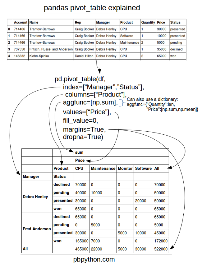
df = pd.read_excel("./data/sales-funnel.xlsx")
df.head(3)

Out[51]:

	Account	Name	Rep	Manager	Product	Quantity	Price	Status
0	714466	Trantow-Barrows	Craig Booker	Debra Henley	CPU	1	30000	presented
1	714466	Trantow-Barrows	Craig Booker	Debra Henley	Software	1	10000	presented
2	714466	Trantow-Barrows	Craig Booker	Debra Henley	Maintenance	2	5000	pending

In [52]:

df["Status"] = df["Status"].astype("category")
df["Status"].cat.set_categories(["won","pending","presented","declined"],inplace=True)
df.info()

<class 'pandas.core.frame.DataFrame'>
RangeIndex: 17 entries, 0 to 16
Data columns (total 8 columns):
Account     17 non-null int64
Name        17 non-null object
Rep         17 non-null object
Manager     17 non-null object
Product     17 non-null object
Quantity    17 non-null int64
Price       17 non-null int64
Status      17 non-null category
dtypes: category(1), int64(3), object(4)
memory usage: 1.2+ KB

In [53]:

pd.pivot_table(df, index = ["Name","Rep","Manager"])

Out[53]:

			Account	Price	Quantity
Name	Rep	Manager
Barton LLC	John Smith	Debra Henley	740150.0	35000.0	1.000000
Fritsch, Russel and Anderson	Craig Booker	Debra Henley	737550.0	35000.0	1.000000
Herman LLC	Cedric Moss	Fred Anderson	141962.0	65000.0	2.000000
Jerde-Hilpert	John Smith	Debra Henley	412290.0	5000.0	2.000000
Kassulke, Ondricka and Metz	Wendy Yule	Fred Anderson	307599.0	7000.0	3.000000
Keeling LLC	Wendy Yule	Fred Anderson	688981.0	100000.0	5.000000
Kiehn-Spinka	Daniel Hilton	Debra Henley	146832.0	65000.0	2.000000
Koepp Ltd	Wendy Yule	Fred Anderson	729833.0	35000.0	2.000000
Kulas Inc	Daniel Hilton	Debra Henley	218895.0	25000.0	1.500000
Purdy-Kunde	Cedric Moss	Fred Anderson	163416.0	30000.0	1.000000
Stokes LLC	Cedric Moss	Fred Anderson	239344.0	7500.0	1.000000
Trantow-Barrows	Craig Booker	Debra Henley	714466.0	15000.0	1.333333

In [54]:

pd.pivot_table(df,
               index = ["Manager","Rep"])

Out[54]:

		Account	Price	Quantity
Manager	Rep
Debra Henley	Craig Booker	720237.0	20000.000000	1.250000
	Daniel Hilton	194874.0	38333.333333	1.666667
	John Smith	576220.0	20000.000000	1.500000
Fred Anderson	Cedric Moss	196016.5	27500.000000	1.250000
Fred Anderson	Wendy Yule	614061.5	44250.000000	3.000000

In [55]:

pd.pivot_table(df,
               index  = ["Manager","Rep"], 
               values = ["Price"])

Out[55]:

		Price
Manager	Rep
Debra Henley	Craig Booker	20000.000000
	Daniel Hilton	38333.333333
	John Smith	20000.000000
Fred Anderson	Cedric Moss	27500.000000
Fred Anderson	Wendy Yule	44250.000000

In [56]:

pd.pivot_table(df,
               index   = ["Manager","Rep"],
               values  = ["Price"],
               aggfunc = [np.sum, len, np.mean])  # np.sum 1개만도 가능

Out[56]:

		sum	len	mean
		Price	Price	Price
Manager	Rep
Debra Henley	Craig Booker	80000	4	20000.000000
	Daniel Hilton	115000	3	38333.333333
	John Smith	40000	2	20000.000000
Fred Anderson	Cedric Moss	110000	4	27500.000000
Fred Anderson	Wendy Yule	177000	4	44250.000000

In [57]:

pd.pivot_table(df,
               index   = ["Manager","Rep"],
               values  = ["Price"],
               columns = ["Product"],
               aggfunc = [np.sum])

Out[57]:

		sum
		Price
	Product	CPU	Maintenance	Monitor	Software
Manager	Rep
Debra Henley	Craig Booker	65000.0	5000.0	NaN	10000.0
	Daniel Hilton	105000.0	NaN	NaN	10000.0
	John Smith	35000.0	5000.0	NaN	NaN
Fred Anderson	Cedric Moss	95000.0	5000.0	NaN	10000.0
Fred Anderson	Wendy Yule	165000.0	7000.0	5000.0	NaN

In [58]:

pd.pivot_table(df,
               index   = ["Manager","Rep"],
               values  = ["Price"],
               columns = ["Product"],
               aggfunc = [np.sum],
               fill_value = 0)

Out[58]:

		sum
		Price
	Product	CPU	Maintenance	Monitor	Software
Manager	Rep
Debra Henley	Craig Booker	65000	5000	0	10000
	Daniel Hilton	105000	0	0	10000
	John Smith	35000	5000	0	0
Fred Anderson	Cedric Moss	95000	5000	0	10000
Fred Anderson	Wendy Yule	165000	7000	5000	0

In [59]:

pd.pivot_table(df,
               index      = ["Manager","Rep"],
               values     = ["Price","Quantity"],
               columns    = ["Product"],
               aggfunc    = [np.sum],
               fill_value = 0)

Out[59]:

		sum
		Price				Quantity
	Product	CPU	Maintenance	Monitor	Software	CPU	Maintenance	Monitor	Software
Manager	Rep
Debra Henley	Craig Booker	65000	5000	0	10000	2	2	0	1
	Daniel Hilton	105000	0	0	10000	4	0	0	1
	John Smith	35000	5000	0	0	1	2	0	0
Fred Anderson	Cedric Moss	95000	5000	0	10000	3	1	0	1
Fred Anderson	Wendy Yule	165000	7000	5000	0	7	3	2	0

In [60]:

pd.pivot_table(df,
               index      = ["Manager", "Rep", "Product"],
               values     = ["Price",   "Quantity"],
               aggfunc    = [np.sum, np.mean],
               fill_value = 0)

Out[60]:

			sum		mean
			Price	Quantity	Price	Quantity
Manager	Rep	Product
Debra Henley	Craig Booker	CPU	65000	2	32500	1.0
		Maintenance	5000	2	5000	2.0
		Software	10000	1	10000	1.0
	Daniel Hilton	CPU	105000	4	52500	2.0
	Daniel Hilton	Software	10000	1	10000	1.0
	John Smith	CPU	35000	1	35000	1.0
	John Smith	Maintenance	5000	2	5000	2.0
Fred Anderson	Cedric Moss	CPU	95000	3	47500	1.5
		Maintenance	5000	1	5000	1.0
		Software	10000	1	10000	1.0
	Wendy Yule	CPU	165000	7	82500	3.5
		Maintenance	7000	3	7000	3.0
		Monitor	5000	2	5000	2.0

In [61]:

pd.pivot_table(df,index   = ["Manager","Rep","Product"],
               values     = ["Price","Quantity"],
               aggfunc    = [np.sum,np.mean],
               fill_value = 0,
               margins    = True)

Out[61]:

			sum		mean
			Price	Quantity	Price	Quantity
Manager	Rep	Product
Debra Henley	Craig Booker	CPU	65000	2	32500	1.000000
		Maintenance	5000	2	5000	2.000000
		Software	10000	1	10000	1.000000
	Daniel Hilton	CPU	105000	4	52500	2.000000
	Daniel Hilton	Software	10000	1	10000	1.000000
	John Smith	CPU	35000	1	35000	1.000000
	John Smith	Maintenance	5000	2	5000	2.000000
Fred Anderson	Cedric Moss	CPU	95000	3	47500	1.500000
		Maintenance	5000	1	5000	1.000000
		Software	10000	1	10000	1.000000
	Wendy Yule	CPU	165000	7	82500	3.500000
		Maintenance	7000	3	7000	3.000000
		Monitor	5000	2	5000	2.000000
All			522000	30	30705	1.764706