
mlcourse.ai – Open Machine Learning Course
Author: Irina Knyazeva, ODS Slack nickname: iknyazeva
Solar flares forecasting (ML approach)
Research plan - Dataset and features description - Exploratory data analysis - Visual analysis of the features - Patterns, insights, pecularities of data - Data preprocessing - Feature engineering and description - Cross-validation, hyperparameter tuning - Validation and learning curves - Prediction for hold-out and test samples - Model evaluation with metrics description - Conclusions
Part 1. What is the solar flares and why we need forecast them?
The sun produces solar flares, which have the power to affect the Earth and near-Earth environment with their great bursts of electromagnetic energy and particles. These flares have the power to blow out transformers on power grids and disrupt satellite systems. There is a long lasting task of predictions such events for minimizing its negative impact. Doing so is a difficult task because of the rarity of these events. The success in this task not changes significantly over the last 60 years. Actually, this was a topic of my Ph.D. research, and I did it without any machine learning. But either in the era of big data, there is no big success in this task. The most common approach described in the paper Bobra et al., 2014. The main drawback of the approach is ignoring time dependence on features. Here I tried to use knowledge about working with time series in features. All data for this project could be downloaded from the [link]
Picture of the sun
Below the picture of our Sun in one of spectral lines $ H_\alpha $, the most beautifull one) You can see bright regions on the Sun surface, these regions called Sun active regions, and in most cases solar flares erased from such region. There is a great site (https://solarmonitor.org/) where is information about the Sun aggregated. Let's look at the Sun and there active regions
import matplotlib.image as mpimg
import wget
import os
import warnings
warnings.filterwarnings("ignore")
import matplotlib.pyplot as plt
%matplotlib inline
#посмотрим на размеченную картинку с solarmonitor
file_url = 'https://solarmonitor.org/data/2014/05/14/pngs/bbso/bbso_halph_fd_20140514_053834.png'
DOWNLOAD = True
IMG_PATH = '../../img/'
file_name = file_url.split(sep='/')[-1]

if DOWNLOAD:
    file_name = wget.download(file_url, out = os.path.join(IMG_PATH, file_name))
    img=mpimg.imread(file_name)
else:
    img=mpimg.imread(os.path.join(IMG_PATH, file_name))
plt.figure(figsize = (12,12))
imgplot = plt.imshow(img)
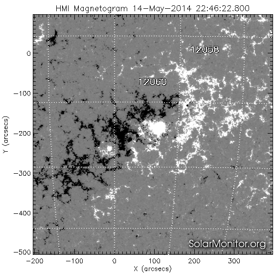
Active regions
Active regions called active because the strength of magnetic field in this regions. Strength of magnetics fields could be taken from so-called solar magnetograms. Magnetogramm of full solar disk at the same time at the next pictures.
#посмотрим на размеченную картинку с solarmonitor
file_url = 'https://solarmonitor.org/data/2014/05/14/pngs/shmi/shmi_maglc_fd_20140514_224622.png'
DOWNLOAD = True
IMG_PATH = '../../img/'
file_name = file_url.split(sep='/')[-1]

if DOWNLOAD:
    file_name = wget.download(file_url, out = os.path.join(IMG_PATH, file_name))
    img=mpimg.imread(file_name)
else:
    img=mpimg.imread(os.path.join(IMG_PATH, file_name))
plt.figure(figsize = (12,12))
imgplot = plt.imshow(img)
A solar flare occurs when magnetic energy that has built up in the solar atmosphere is suddenly released. Solar flares are an often occurrence when the Sun is active in the years around solar maximum. Many solar flares can occur on just one day during this period! Around solar minimum, solar flares might occur less than once per week.
The classification of solar flares
Solar flares are classified as A (smallest), B, C, M or X (strongest) according to the peak flux (in watts per square metre, W/m2) of 1 to 8 Ångströms X-rays near Earth, as measured by XRS instrument on-board the GOES-15 satellite which is in a geostationary orbit over the Pacific Ocean. Some (mostly stronger) solar flares can launch huge clouds of solar plasma into space which we call a coronal mass ejection. When a coronal mass ejection arrives at Earth, it can cause a geomagnetic storm and intense auroral displays.
Solar flares prediction
Most of techniques are based on the complexity of the photospheric magnetic field of the Sun's active regions. There are a large number of dif- ferent characteristics that can be used for magnetic field complexity description. Due to many empirical assumptions during their calculation, they are hardly reproducible. For HMI/SDO vector magnetograms an automated active region tracking system exist called Spaceweather HMI Active Region Patch SHARP. For each active region, key features called SHARP parameters were calculated and are available online. Computation of these features is based on SDO vector magnetograms .
One example of Active region at the picture below:
Data description
To define a solar flare, we only consider flares with a Geostationary Operational Environmental Satellite (GOES) X-ray flux peak magnitude above the M1.0 level. This allows us to focus only on major flares. For the purposes of this study, we defined a positive event to be an active region that flares with a peak magnitude above the M1.0 level, as defined by the GOES database. A negative event would be an active region that does not have such an event within a 24-hour time span. For collection active region for the negative class, we will gather also information about all regions where X-ray flux peak magnitude above the C1.0 level. So in our training set the same active region could be positive in one time and negative in the other. In each time moment, our target value will be 1 if in the next 24 hours will be the event with flux above the M1.0 level and 0 if not.
For doing that we need to describe the complexity of each active region with the features. I (and most other researchers) did it with so-called SHARP features.
The Solar Dynamic's Observatory's Helioseismic and Magnetic Imager is the first instrument to continuously map the vector magnetic field of the sun. The SDO takes the most data of any NASA satellite in history, approximately 2 terabytes per day, making it an ideal dataset for such a problem. Using this data, we can characterize active regions on the sun. From the time frame of 2010 May to 2018 December, we focused on 18 parameters calculated using the SHARP vector magnetic field data. They characterize various physical and geometrical qualities of the active region.
- USFLUX is the total unsigned flux.
- MEANGAM is the mean angle of field from radial.
- MEANGBT is the mean gradient of total field.
- MEANGBZ is the mean gradient of vertical field.
- MEANGBH is the mean gradient of the horizontal field.
- MEANJZD is the mean vertical current density.
- TOTUSJZ is the total unsigned vertical current.
- MEANALP is the mean characteristic twist parameter.
- MEANJZH is the mean current helicity.
- TOTUSJH is the total unsigned vertical current.
- ABSNJZH is the absolute value of the net current helicity.
- SAVNCPP is the sum of the modulus of the net current per polarity.
- MEANPOT is the mean photospheric magnetic free energy.
- TOTPOT is the total photospheric magnetic free energy density.
- MEANSHR is the mean shear angle.
- SHRGT45 is the fraction of area with shear greater than 45 degrees.
- R_VALUE is the sum of flux near polarity inversion line.
- AREA_ACR is the area of strong field pixels in the active region.
The following section of code initializes the start and end dates of the data set used in this study and also fetches the set of possible positive events and the mapper from NOAA active region numbers to the HARPNUMs used in our database.
Get all info about solar flares from goes
This part contain code for gathering solar data. Here data from two instruments collected: goes and SDO. There is special package sunpy for handling solar data.
#pip install sunpy
#pip install suds-py3
#pip install drms
from datetime import timedelta
import datetime
import sunpy
from sunpy.time import TimeRange
from sunpy.instr import goes
import numpy as np
import pandas as pd
DOWNLOAD = False
DATA_PATH = '../../data/solar_flares'
if DOWNLOAD:
    time_range = TimeRange('2010/06/01 00:10', '2018/12/01 00:20')
    #time_range = TimeRange(t_start,t_end)
    goes_events = goes.get_goes_event_list(time_range,'C1')
    goes_events = pd.DataFrame(goes_events)
else:
    goes_events = pd.read_csv(os.path.join(DATA_PATH,'goes_events_2010_2018.csv'), index_col=[0])
goes_events['noaa_active_region'] = goes_events['noaa_active_region'].replace(0,np.nan)
goes_events.dropna(inplace=True)
goes_events.drop(['goes_location','event_date','end_time','peak_time'], axis=1, inplace=True)
goes_events.start_time = goes_events.start_time.astype('datetime64[ns]')
goes_events.head()
Active regions detections
There are different approaches to active regions detections. One of them with manual correction and done each day in NOAA. Active regions in this catalog have NOAA numbers. The team of SDO has own fully automated system of AR detections, and their regions called HARPs. Also, they compute plenty of parameters of magnetic field complexity. So I used harp regions with features, but information about goes flux there is only for NOAA regions. HARP and NOAA regions are not coinciding, but there is the mapping between this two catalogs. Below the code for mapping between the HARP and NOAA regions.
#download mapper NOAA
if os.path.isfile(os.path.join(DATA_PATH,'all_harps_with_noaa_ars.txt')):
    num_mapper = pd.read_csv(os.path.join(DATA_PATH,'all_harps_with_noaa_ars.txt'), sep=' ',index_col=[0])
else:
    num_mapper = pd.read_csv('http://jsoc.stanford.edu/doc/data/hmi/harpnum_to_noaa/all_harps_with_noaa_ars.txt',sep=' ')
    num_mapper.to_csv(os.path.join(DATA_PATH,'all_harps_with_noaa_ars.txt'), sep=' ')
num_mapper.tail()
def convert_noaa_to_harpnum(noaa_ar):
    """
    Converts from a NOAA Active Region to a HARPNUM
    Returns harpnum if present, else None if there are no matching harpnums

    Args:
    """
    idx = num_mapper[num_mapper['NOAA_ARS'].str.contains(str(int(noaa_ar)))]
    return None if idx.empty else int(idx.HARPNUM.values[0])
goes_events['harp_number'] = goes_events['noaa_active_region'].apply(convert_noaa_to_harpnum)
goes_events.dropna(inplace=True)
Events class could be mapped to flux, which is continuous. It could be done with method flareclass_to_flux from goes
#Goes class flares better convert to flux value. It could be done with method flareclass_to_flux from goes
goes_events['flux'] =  goes_events['goes_class'].apply(lambda x: 1e06*goes.flareclass_to_flux(x).value)
goes_events.head()
In one region could be many flares of differents classes. We have more then 1300 events and only Let's see to the countplot for the harp_number
import seaborn as sns
sns.countplot(x='harp_number', data = goes_events)
Loading data
Data with the main features of Active regions could be taken from SDO database. There is a special package for acesssing data drms. We will download meta information with the all keywords with drms
#here list of keywords we want to download. Keywords computed for harp regions.
#Here we walk through the all harp regions, download features and save them to disk (it is very time consuming)
import drms
c = drms.Client()
list_keywords = ['T_REC,CRVAL1,CRLN_OBS,USFLUX,MEANGBT,MEANJZH,MEANPOT,SHRGT45,TOTUSJH,MEANGBH,MEANALP,MEANGAM,MEANGBZ,MEANJZD,TOTUSJZ,SAVNCPP,TOTPOT,MEANSHR,AREA_ACR,R_VALUE,ABSNJZH']
harp_list = pd.unique(goes_events.harp_number)
for harp in harp_list:
    str_query = f'hmi.sharp_cea_720s[{str(int(harp))}]'

    if os.path.isfile(os.path.join(DATA_PATH+'/keys_regions',str_query+'.csv')):
        print(f'Harp number {harp} already exist\n')
    else:
        print(f'load region with Harp number {harp}')
        keys = c.query(str_query, key=list_keywords)
        keys.to_csv(os.path.join(DATA_PATH+'/keys_regions',str_query+'.csv'))
Part 2. Exploratory data analysis
Now there are many CSV files for each harp region and we can analyze the evolution of different parameters with the time. It is believed that before the flares complexity of magnetic field changes and there are special patterns in features evolutions.
def plot_harp_features_flares(harp, goes_events = goes_events, DATA_PATH=DATA_PATH, feature_key = 'R_VALUE'):
    str_query = f'hmi.sharp_cea_720s[{str(int(harp))}]'
    df = pd.read_csv(os.path.join(DATA_PATH+'/keys_regions',str_query+'.csv'), index_col=[0])
    df['T_REC']  = drms.to_datetime(df.T_REC)
    df.set_index('T_REC', inplace=True)
    first_date = df.index.get_values()[0]

    is_visible =  abs(df['CRVAL1']-df['CRLN_OBS'])<60
    df = df[is_visible]

    flux = goes_events[goes_events['harp_number']==harp][['start_time','flux']].set_index('start_time')
    #plt.figure(figsize = (10,14))
    fig, ax1 = plt.subplots(figsize=(15,5))
    #ax1.figure(figsize = (10,14))
    first_date = flux.index.get_values()[0]
    first_date = df.index.get_values()[0]
    #t2 = flux.index.get_values()[0]
    #first_data = min(t1,t2)
    dates_to_show = pd.date_range(pd.Timestamp(first_date).strftime('%m/%d/%Y'), periods=14, freq='d')
    labels = dates_to_show.strftime('%b %d')
    color = 'tab:green'
    ax1.plot(df.index, df[feature_key], color=color)
    ax2 = ax1.twinx()
    ax2.bar(flux.index, flux.flux, width=0.05, facecolor='indianred')
    plt.setp(ax1, xticks=dates_to_show, xticklabels=labels);
    #ax2.set_ylim(0,10)
harp = 6327
plot_harp_features_flares(harp, feature_key = 'R_VALUE')
Features from csv
Now we need to generate features from time series evolutions. It is believed that active region "prepared for giving a flare". So I decided to take complexity features at the considered moment add aggregates from the past 1. Features at the time moment, not all moments each 2 hours 2. Mean and range (max-min) for features at the last 2 hours 3. Mean and range (max-min) at the last 6 hours 4. Mean and range (max-min) at the last 12 hours 5. Mean and range (max-min) at the last 24 hours 6. Mean and range (max-min) at the last 48 hours
Also there are instrumental distortion if angle between observer and the point at the sun big, usually records where latituted more than 70 is droped from estimation.
def extract_features_from_csv(harp, time_stamp = 2, delay_hours = [2,6,12,24,48], long=70):
    """
    process downloaded csv files with time series features and create features from them
    harp: harp number
    time_stamp: frequence
    delay_hour:
    return: data_frame with features
    """

    str_query = f'hmi.sharp_cea_720s[{str(int(harp))}]'
    df = pd.read_csv(os.path.join(DATA_PATH+'/keys_regions',str_query+'.csv'), index_col=[0])
    df['T_REC']  = drms.to_datetime(df.T_REC)
    df.set_index('T_REC', inplace=True)
    is_visible =  abs(df['CRVAL1']-df['CRLN_OBS'])<long
    df = df[is_visible].drop(['CRVAL1','CRLN_OBS'], axis=1)
    first_date = df.index.get_values()[0]
    last_date = df.index.get_values()[-1]
    first_date = first_date+np.timedelta64(1, 'D')
    #round to closet whole hour
    first_date = pd.to_datetime(first_date).replace(microsecond=0,second=0,minute=0)+timedelta(hours=1)

    t_range = pd.date_range(first_date, last_date, freq=str(time_stamp)+'H')
    df_orig = df.loc[t_range]
    df_list = []
    df_list.append(df_orig)
    for delay in delay_hours:
        columns_=[col+'_mean_'+str(delay) for col in df_orig.columns]
        df_delay = df.rolling(str(delay)+'h').mean()
        df_delay.columns = columns_
        df_delay = df_delay.loc[t_range]
        df_list.append(df_delay)
        columns_=[col+'_range_'+str(delay) for col in df_orig.columns]
        df_delay = df.rolling(str(delay)+'h').max() - df.rolling(str(delay)+'h').min()
        df_delay.columns = columns_
        df_delay = df_delay.loc[t_range]
        df_list.append(df_delay)
    full_df = pd.concat(df_list, axis=1)
    full_df.dropna(inplace=True)
    full_df['HARP']=harp
    return full_df
harp = harp_list[4]
full_df = extract_features_from_csv(harp)
full_df.head()
Define target
At each active region (harp) at each moment targer will be the number of events where flux exceed M1.0 level (or 10 in flux value) in any time in the next 24 hours and 0 when there is not such events. Actually I will predict only the fact of solar flares, but maybe in future this information will be usefull, especially on error analysis stage
def compute_target(full_df, goes_events=goes_events, horizont = 24, level = 10):
    harp = full_df['HARP'][0]
    big_events = goes_events[(goes_events['harp_number']==harp) &(goes_events.flux>level)]
    target = pd.Series(full_df.index.map(lambda x: np.sum((x>big_events.start_time - np.timedelta64(horizont,'h'))
           & (x<big_events.start_time))))
    full_df['target'] = target.values
    return full_df
full_df=compute_target(full_df)
Feature from goes history
Also it is seemed usefull to account previous activity in the active region. Here I sum all previous activity up to the considered moment
def compute_prev_flux(full_df, goes_events=goes_events):
    harp = full_df['HARP'][0]

    goes_harp = goes_events[(goes_events['harp_number']==harp)]
    prev_flux  = pd.Series(full_df.index.map(lambda x: goes_harp.loc[goes_harp.start_time<x].flux.sum()))
    full_df['prev_flux'] = prev_flux.values
    return full_df
full_df=compute_prev_flux(full_df)
full_df.head()
from tqdm import tqdm
DOWNLOAD = False
if DOWNLOAD and os.path.isfile(os.path.join(DATA_PATH, 'solar_train.pkl')):
    train_df  = pd.read_pickle(os.path.join(DATA_PATH, 'solar_train.pkl'))
else:
    df_list=[]
    for harp in tqdm(harp_list):
        df_ = extract_features_from_csv(harp)
        if df_.shape[0]==0:
            continue
        df_ = compute_target(df_, goes_events=goes_events)
        df_ = compute_prev_flux(df_)
        df_['Time'] = df_.index
        df_list.append(df_)
    train_df = pd.concat(df_list, ignore_index=True).sort_values(by = 'Time')
    train_df.to_pickle(os.path.join(DATA_PATH, 'solar_train.pkl'))
train_df.target.value_counts()
train_df['bin_target'] = train_df.target.map(lambda x: 0 if x==0 else 1)
train_df['bin_target'].value_counts()
Let's see how the main features (without aggregates) depends with each other and with the target
key_cols = str.split('USFLUX,MEANGBT,MEANJZH,MEANPOT,SHRGT45,TOTUSJH,MEANGBH,MEANALP,MEANGAM,MEANGBZ,MEANJZD,TOTUSJZ,SAVNCPP,TOTPOT,MEANSHR,AREA_ACR,R_VALUE,ABSNJZH', sep=',')
sns.set(rc={'figure.figsize':(12.7,10.27)})
sns.heatmap(train_df[key_cols].corr(), annot=True)
sns.pairplot( train_df, vars=key_cols[:3],
             diag_kind='kde',hue='bin_target', markers="+", aspect=1.5);
sns.pairplot( train_df, vars=key_cols[3:6],
             diag_kind='kde',hue='bin_target', markers="+", aspect=1.5);
sns.pairplot( train_df, vars=key_cols[6:9],
             diag_kind='kde',hue='bin_target', markers="+", aspect=1.5);
sns.pairplot( train_df, vars=key_cols[9:12],
             diag_kind='kde',hue='bin_target', markers="+", aspect=1.5);
sns.pairplot( train_df, vars=key_cols[12:15],
             diag_kind='kde',hue='bin_target', markers="+", aspect=1.5);
sns.pairplot( train_df, vars=key_cols[15:18],
             diag_kind='kde',hue='bin_target', markers="+", aspect=1.5);
g = sns.FacetGrid(train_df, hue="bin_target", height=4)
g.map(sns.distplot, 'prev_flux')
Part 5. Data preprocessing. Metric selection and model selection
This is a binary classification problem with highly unbalances data. In practice, if we want to safe space objects from damages it is more important to reveal all cases, so we will watch to recall as a metric, but in cross-validation roc_auc as a more balanced metric will be used.
For holdout set I leave all 2017 and 2018 year. But actually, we could update the model in real time and such splitting not so important.
For cross_validation I will use time series split, in other cases I'll get data leakage, through 24 hours I will definitely now about flare
As a model, I start with logistic regression as a baseline, try random forest and lighgbm.
from sklearn.preprocessing import StandardScaler
from sklearn.model_selection import TimeSeriesSplit, cross_val_score, GridSearchCV
from sklearn.metrics import roc_auc_score, recall_score, precision_score, accuracy_score, classification_report, confusion_matrix
from sklearn.linear_model import LogisticRegression
from sklearn.pipeline import Pipeline
from sklearn.ensemble import RandomForestClassifier
#create Year feature
train_df['Year'] = train_df.Time.dt.year
train_part = train_df.loc[~train_df['Year'].isin([2017,2018])]
test_part = train_df.loc[train_df['Year'].isin([2017,2018])]
train_part.bin_target.value_counts()
test_part.bin_target.value_counts()
So we have 2907 positive events in train set and 109 in test. Try to fit baseline model only with key features without aggregates
tcv = TimeSeriesSplit(n_splits=10)
logit_pipe = Pipeline([('scaler', StandardScaler()), ('logit', LogisticRegression(class_weight='balanced', random_state=17))])
score = cross_val_score(logit_pipe, train_part[key_cols], train_part['bin_target'], cv=tcv, scoring = 'roc_auc')
print('Validation score:', score)
logit_pipe.fit(train_part[key_cols], train_part['bin_target'])
Actually not so bad, let's see at the confusion matrix at the train and test part.
y_pred = logit_pipe.predict_proba(train_part[key_cols])
class_names = ['No Flare', 'Flare']
pd.DataFrame(confusion_matrix(train_part['bin_target'],y_pred[:,1]>0.5), index=class_names, columns=class_names)
y_pred = logit_pipe.predict_proba(test_part[key_cols])
class_names = ['No Flare', 'Flare']
pd.DataFrame(confusion_matrix(test_part['bin_target'],y_pred[:,1]>0.5), index=class_names, columns=class_names)
So we missed 11 flares at the test set, and 432 in train set. Let's try Random Forest from the box
%%time
rf = RandomForestClassifier(n_estimators = 100, max_depth=3, class_weight='balanced')
score = cross_val_score(rf, train_part[key_cols], train_part['bin_target'], cv=tcv, scoring = 'roc_auc')
print('Validation score:', score)
%%time
rf = RandomForestClassifier(n_estimators = 500,  max_depth=3, class_weight='balanced')
rf.fit(train_part[key_cols], train_part['bin_target'])
rf_pred = rf.predict_proba(train_part[key_cols])
class_names = ['No Flare', 'Flare']
pd.DataFrame(confusion_matrix(train_part['bin_target'],rf_pred[:,1]>0.5), index=class_names, columns=class_names)
rf_pred = rf.predict_proba(test_part[key_cols])
class_names = ['No Flare', 'Flare']
pd.DataFrame(confusion_matrix(test_part['bin_target'],rf_pred[:,1]>0.5), index=class_names, columns=class_names)
import lightgbm as lgb
%%time
lg = lgb.LGBMClassifier(n_estimators=300, max_depth=5, num_leaves=10)
tcv = TimeSeriesSplit(n_splits=10)
score = cross_val_score(lg, train_part[key_cols], train_part['bin_target'], cv=tcv, scoring = 'roc_auc')
print('Validation score:', score)
lg = lgb.LGBMClassifier(n_estimators=500, max_depth=5, num_leaves=10)
lg.fit(train_part[key_cols], train_part['bin_target'])
lg_pred = lg.predict_proba(train_part[key_cols])
class_names = ['No Flare', 'Flare']
pd.DataFrame(confusion_matrix(train_part['bin_target'],lg_pred[:,1]>0.5), index=class_names, columns=class_names)
lg_pred = lg.predict_proba(test_part[key_cols])
class_names = ['No Flare', 'Flare']
pd.DataFrame(confusion_matrix(test_part['bin_target'],lg_pred[:,1]>0.5), index=class_names, columns=class_names)
Lightgbm with this parameters give us less false positive alarms, but very low recall
Part 6. Feature engineering and description
Actually all features enineering was done before, it is historical features, previous flux, here we try to use them and add Year as a feature, because there is a 11 year cycle in solar activity. Number of flares changes significantly from year to year.
#number of flares by years
train_df.groupby('Year')['bin_target'].count()
from sklearn.preprocessing import OneHotEncoder
from sklearn.compose import ColumnTransformer
#ohe = OneHotEncoder(sparse=False,handle_unknown='ignore')
cat_cols = ['Year']
idx_split = train_part.shape[0]
%%time
tcv = TimeSeriesSplit(n_splits=10)
num_cols = key_cols+['prev_flux']
train_ohe = pd.concat([pd.get_dummies(train_df['Year'], prefix = 'Year'), train_df[num_cols]], axis=1)
transformers = [('num', StandardScaler(), num_cols)]
ct = ColumnTransformer(transformers=transformers, remainder = 'passthrough' )
logit_pipe = Pipeline([('transform', ct), ('logit', LogisticRegression(C=1, class_weight='balanced', random_state=17))])
score = cross_val_score(logit_pipe, train_ohe.loc[:idx_split,:], train_df.loc[:idx_split,'bin_target'], cv=tcv, scoring = 'roc_auc')
print('Validation score:', score)
Lets try to add delay features for 24 hours, range for example
%%time
tcv = TimeSeriesSplit(n_splits=10)
delay=24
col_range=[col+'_range_'+str(delay) for col in key_cols]
num_cols = key_cols+['prev_flux']+col_range
transformers = [('num', StandardScaler(), num_cols)]
ct = ColumnTransformer(transformers=transformers, remainder = 'passthrough' )
train_ohe = pd.concat([pd.get_dummies(train_df['Year'], prefix = 'Year'), train_df[num_cols]], axis=1)
logit_pipe = Pipeline([('transform', ct), ('logit', LogisticRegression(C=1, class_weight='balanced', random_state=17))])
score = cross_val_score(logit_pipe, train_ohe.loc[:idx_split,:], train_df.loc[:idx_split,'bin_target'], cv=tcv, scoring = 'roc_auc')
print('Validation score:', score)
Don't see any improvement, so I try will tune logistic with base features and lightgbm on the whole dataset. Random Forest will be later
Part 7. Cross-validation, hyperparameter tuning
%%time
tcv = TimeSeriesSplit(n_splits=5)
num_cols = key_cols+['prev_flux']
train_ohe = pd.concat([pd.get_dummies(train_df['Year'], prefix = 'Year'), train_df[num_cols]], axis=1)
transformers = [('num', StandardScaler(), num_cols)]
ct = ColumnTransformer(transformers=transformers, remainder = 'passthrough' )
logit_pipe = Pipeline([('transform', ct), ('logit', LogisticRegression(C=1, class_weight='balanced', random_state=17))])

param_grid = {
    'logit__C': [.5, 1.0, 2.0, 10.0]
    }
gs = GridSearchCV(logit_pipe, param_grid, cv=tcv, scoring = 'roc_auc', n_jobs = -1)
gs.fit(train_ohe.loc[:idx_split,:], train_df.loc[:idx_split,'bin_target'])
pd.DataFrame(gs.cv_results_)[['params','mean_test_score', 'std_test_score', 'mean_train_score']]
%%time
tcv = TimeSeriesSplit(n_splits=5)
num_cols = key_cols+['prev_flux']
train_ohe = pd.concat([pd.get_dummies(train_df['Year'], prefix = 'Year'), train_df[num_cols]], axis=1)
transformers = [('num', StandardScaler(), num_cols)]
ct = ColumnTransformer(transformers=transformers, remainder = 'passthrough' )
logit_pipe = Pipeline([('transform', ct), ('logit', LogisticRegression(C=1, class_weight='balanced', random_state=17))])

param_grid = {
    'logit__C': [0.01, 0.025,0.05,.1,0.15,0.2,0.3,0.4]
    }
gs = GridSearchCV(logit_pipe, param_grid, cv=tcv, scoring = 'roc_auc', n_jobs = -1)
gs.fit(train_ohe.loc[:idx_split,:], train_df.loc[:idx_split,'bin_target'])
pd.DataFrame(gs.cv_results_)[['params','mean_test_score', 'std_test_score', 'mean_train_score']]
%%time
tcv = TimeSeriesSplit(n_splits=10)
num_cols = key_cols+['prev_flux']
train_ohe = pd.concat([pd.get_dummies(train_df['Year'], prefix = 'Year'), train_df[num_cols]], axis=1)
transformers = [('num', StandardScaler(), num_cols)]
ct = ColumnTransformer(transformers=transformers, remainder = 'passthrough' )
logit_pipe = Pipeline([('transform', ct), ('logit', LogisticRegression(C=0.01, class_weight='balanced', random_state=17))])
score = cross_val_score(logit_pipe, train_ohe.loc[:idx_split,:], train_df.loc[:idx_split,'bin_target'], cv=tcv, scoring = 'roc_auc', n_jobs=-1)
print('Validation score:', score)
Tuning lightgbm (ohe features)
import lightgbm as lgb
tcv = TimeSeriesSplit(n_splits=10)
delay=24
col_range=[col+'_range_'+str(delay) for col in key_cols]
col_mean = [col+'_mean_'+str(delay) for col in key_cols]
num_cols = key_cols+['prev_flux']+col_range+col_mean
transformers = [('num', StandardScaler(), num_cols)]
ct = ColumnTransformer(transformers=transformers, remainder = 'passthrough' )
train_ohe = pd.concat([pd.get_dummies(train_df['Year'], prefix = 'Year'), train_df[num_cols]], axis=1)
#score = cross_val_score(logit_pipe, train_ohe.loc[:idx_split,:], train_df.loc[:idx_split,'bin_target'], cv=tcv, scoring = 'roc_auc')
#print('Validation score:', score)
%%time
lg = lgb.LGBMClassifier(silent=False)
param_dist = {"max_depth": [5,10,15,20],
              "num_leaves": [5,10,20,30],
              "n_estimators": [300],
              #"learning_rate" : [0.1,0.05]
             }
grid_search = GridSearchCV(lg, n_jobs=-1, param_grid=param_dist, cv = tcv, scoring="roc_auc", verbose=5)
grid_search.fit(train_ohe.loc[:idx_split,:], train_df.loc[:idx_split,'bin_target'])
pd.DataFrame(grid_search.cv_results_)[['params','mean_test_score', 'std_test_score', 'mean_train_score']]
pd.DataFrame(grid_search.cv_results_)[['params','mean_test_score', 'std_test_score', 'mean_train_score']].iloc[1,0]
lg = lgb.LGBMClassifier(silent=False)
param_dist = {"max_depth": [5],
              "num_leaves": [10],
              "n_estimators": [500],
              "learning_rate" : [0.025,0.015, 0.01]
             }
grid_search = GridSearchCV(lg, n_jobs=-1, param_grid=param_dist, cv = 3, scoring="roc_auc", verbose=5)
grid_search.fit(train_ohe.loc[:idx_split,:], train_df.loc[:idx_split,'bin_target'])
pd.DataFrame(grid_search.cv_results_)[['params','mean_test_score', 'std_test_score', 'mean_train_score']]
So for lightgbm final set of parameters param_dist = {"max_depth": [5], "num_leaves": [10], "n_estimators": [500], "learning_rate" : [0.01] }
Part 8. Validation and learning curves
Let's plot learning curve for both models with best parameters
from sklearn.model_selection import learning_curve
tcv = TimeSeriesSplit(n_splits=5)
num_cols = key_cols+['prev_flux']
train_ohe = pd.concat([pd.get_dummies(train_df['Year'], prefix = 'Year'), train_df[num_cols]], axis=1)
transformers = [('num', StandardScaler(), num_cols)]
ct = ColumnTransformer(transformers=transformers, remainder = 'passthrough' )
logit_pipe = Pipeline([('transform', ct), ('logit', LogisticRegression(C=0.01, class_weight='balanced', random_state=17))])
train_sizes, train_scores, test_scores = learning_curve(logit_pipe, train_ohe.loc[:idx_split,:], train_df.loc[:idx_split,'bin_target'],
                                                                       train_sizes=np.arange(0.1,1, 0.2),
                                                                       cv=tcv, scoring='roc_auc', n_jobs=-1)
plt.grid(True)
plt.plot(train_sizes, train_scores.mean(axis = 1), 'g-', marker='o', label='train')
plt.plot(train_sizes, test_scores.mean(axis = 1), 'r-', marker='o', label='test')
plt.ylim((0.0, 1.05))
plt.legend(loc='lower right')
delay=24
col_range=[col+'_range_'+str(delay) for col in key_cols]
col_mean = [col+'_mean_'+str(delay) for col in key_cols]
num_cols = key_cols+['prev_flux']+col_range+col_mean
transformers = [('num', StandardScaler(), num_cols)]
ct = ColumnTransformer(transformers=transformers, remainder = 'passthrough' )
train_ohe = pd.concat([pd.get_dummies(train_df['Year'], prefix = 'Year'), train_df[num_cols]], axis=1)
lg = lgb.LGBMClassifier(silent=False,max_depth=5, num_leaves=10,n_estimators=500,learning_rate=0.01)
train_sizes, train_scores, test_scores = learning_curve(lg, train_ohe.loc[:idx_split,:], train_df.loc[:idx_split,'bin_target'],
                                                                       train_sizes=np.arange(0.1,1, 0.2),
                                                                       cv=tcv, scoring='roc_auc', n_jobs=-1)
plt.grid(True)
plt.plot(train_sizes, train_scores.mean(axis = 1), 'g-', marker='o', label='train')
plt.plot(train_sizes, test_scores.mean(axis = 1), 'r-', marker='o', label='test')
plt.ylim((0.0, 1.05))
plt.legend(loc='lower right')
Learning curves looks OK!
Part 9. Prediction for hold-out and test samples and model evaluation
Now time to fit model on the whole dataset and test it on the hold out
num_cols = key_cols+['prev_flux']
train_ohe = pd.concat([pd.get_dummies(train_df['Year'], prefix = 'Year'), train_df[num_cols]], axis=1)
transformers = [('num', StandardScaler(), num_cols)]
ct = ColumnTransformer(transformers=transformers, remainder = 'passthrough' )
logit_pipe = Pipeline([('transform', ct), ('logit', LogisticRegression(C=0.01, class_weight='balanced', random_state=17))])
logit_pipe.fit(train_ohe.loc[:idx_split,:], train_df.loc[:idx_split,'bin_target'])
logit_pred = logit_pipe.predict_proba(train_ohe.loc[idx_split:,:])
class_names = ['No Flare', 'Flare']
print(roc_auc_score(train_df.loc[idx_split:,'bin_target'],logit_pred[:,1]))
pd.DataFrame(confusion_matrix(train_df.loc[idx_split:,'bin_target'],logit_pred[:,1]>0.5), index=class_names, columns=class_names)
delay=24
col_range=[col+'_range_'+str(delay) for col in key_cols]
col_mean = [col+'_mean_'+str(delay) for col in key_cols]
num_cols = key_cols+['prev_flux']+col_range+col_mean
transformers = [('num', StandardScaler(), num_cols)]
ct = ColumnTransformer(transformers=transformers, remainder = 'passthrough' )
train_ohe = pd.concat([pd.get_dummies(train_df['Year'], prefix = 'Year'), train_df[num_cols]], axis=1)
lg = lgb.LGBMClassifier(silent=False,max_depth=5, num_leaves=10,n_estimators=800,learning_rate=0.01)
lg.fit(train_ohe.loc[:idx_split,:], train_df.loc[:idx_split,'bin_target'])
#lg_pred = lg.predict_proba(train_ohe.loc[idx_split:,:])
class_names = ['No Flare', 'Flare']
lg_pred = lg.predict_proba(train_ohe.loc[idx_split:,:])
pd.DataFrame(confusion_matrix(train_df.loc[idx_split:,'bin_target'],lg_pred[:,1]>0.5), index=class_names, columns=class_names)
Here we can see no false alarm, let's mix them
from sklearn.model_selection import cross_val_predict
tcv = TimeSeriesSplit(n_splits=5)
num_cols = key_cols+['prev_flux']
train_ohe = pd.concat([pd.get_dummies(train_df['Year'], prefix = 'Year'), train_df[num_cols]], axis=1)
transformers = [('num', StandardScaler(), num_cols)]
ct = ColumnTransformer(transformers=transformers, remainder = 'passthrough' )
logit_pipe = Pipeline([('transform', ct), ('logit', LogisticRegression(C=0.01, class_weight='balanced', random_state=17))])
y_pred_logit = cross_val_predict(logit_pipe, train_ohe.loc[:idx_split,:], train_df.loc[:idx_split,'bin_target'], cv=3, method='predict_proba')[:,1]
delay=24
col_range=[col+'_range_'+str(delay) for col in key_cols]
col_mean = [col+'_mean_'+str(delay) for col in key_cols]
num_cols = key_cols+['prev_flux']+col_range+col_mean
transformers = [('num', StandardScaler(), num_cols)]
ct = ColumnTransformer(transformers=transformers, remainder = 'passthrough' )
train_ohe = pd.concat([pd.get_dummies(train_df['Year'], prefix = 'Year'), train_df[num_cols]], axis=1)
lg = lgb.LGBMClassifier(silent=False,max_depth=5, num_leaves=10,n_estimators=800,learning_rate=0.01)
y_pred_lg = cross_val_predict(lg, train_ohe.loc[:idx_split,:], train_df.loc[:idx_split,'bin_target'], cv=3, method='predict_proba')[:,1]
answ = pd.DataFrame(data = np.vstack([y_pred_logit, y_pred_lg,train_df.loc[:idx_split,'bin_target'].values]).T, columns=['logit','lgb','real'])
answ.loc[answ['real']==1].sample(5)
logit_2lev = LogisticRegression()
cross_val_score(logit_2lev, answ.drop('real',axis=1), answ['real'], cv=5, scoring = 'roc_auc')
logit_2lev.fit(answ.drop('real',axis=1), answ['real'])
logit_2lev.coef_/np.sum(logit_2lev.coef_)
y_mixed = 0.73*logit_pred[:,1]+0.27*lg_pred[:,1]
pd.DataFrame(confusion_matrix(train_df.loc[idx_split:,'bin_target'],y_mixed>0.5), index=class_names, columns=class_names)
Part 11. Conclusions
In this task there are plenty of room for improvement, but final result good. Almost all flares was revealed and 10% of false alarm not a big problem