Lecture 1.2. S- and Т-matrix methods¶

This lecture will draw an analogy between the Fresnel and Mie coefficients, introduce scattering and transmission matrices, and review algorithms for calculating the optical properties of multilayer structures with simple boundaries and media reducible to such structures.

Reflection and transmission a plane interfaces¶

In source-free regions in homogeneous isotropic space, the field in Cartesian coordinates can be decomposed into waves of two orthogonal polarisations, ‘s’ and ‘p’, with respect to the Cartesian axis $Z$. The waves are separated along the direction of propagation relative to this axis, which corresponds to two types of solutions of the dispersion equation, and is denoted below by the upper index $\sigma=\pm$. Let us denote the electric field amplitudes of the ‘s’-polarization as $a^{s\sigma}$, and the magnetic field amplitudes of the ‘p’-polarization as $a^{p\sigma}$. Then, from the Faraday's law and the theorem of magnetic field circulation we obtain \begin{align*} \boldsymbol{E}^{s\sigma} &= a^{s\sigma} \hat{\boldsymbol{e}}^{s\sigma} \Rightarrow \boldsymbol{H}^{s\sigma} = \dfrac{1}{\omega\mu}\boldsymbol{k}^{\sigma} \times \boldsymbol{E}^{s\sigma} = \dfrac{k}{\omega\mu} a^{s\sigma} \hat{\boldsymbol{e}}^{p\sigma} \\ \boldsymbol{H}^{p\sigma} &= a^{p\sigma} \hat{\boldsymbol{e}}^{s\sigma} \Rightarrow \boldsymbol{E}^{p\sigma} = -\dfrac{1}{\omega\varepsilon}\boldsymbol{k}^{\sigma} \times \boldsymbol{H}^{p\sigma} = -\dfrac{k}{\omega\varepsilon} a^{p\sigma} \hat{\boldsymbol{e}}^{p\sigma} \end{align*} and the field decomposition in source-free regions writes \begin{equation*} \left( \begin{array}{c} \boldsymbol{E}\left(\boldsymbol{r}\right) \\ \boldsymbol{H}\left(\boldsymbol{r} \right) \end{array} \right) = \iint_{-\infty}^{\infty} dk_{x}dk_{y} e^{i\boldsymbol{\rho}\boldsymbol{\varkappa}} \sum_{\sigma=\pm} \left( \! \begin{array}{c} a^{s\sigma}_{\boldsymbol{k}} \hat{\boldsymbol{e}}^{s\sigma}_{\boldsymbol{k}} - \dfrac{k}{\omega\varepsilon} a^{p\sigma}_{\boldsymbol{k}} \hat{\boldsymbol{e}}^{p\sigma}_{\boldsymbol{k}} \\ a^{p\sigma}_{\boldsymbol{k}} \hat{\boldsymbol{e}}^{s\sigma}_{\boldsymbol{k}} + \dfrac{k}{\omega\mu} a^{s\sigma}_{\boldsymbol{k}} \hat{\boldsymbol{e}}^{p\sigma}_{\boldsymbol{k}} \end{array} \! \right) e^{\sigma ik_{z}z} \end{equation*} where $\boldsymbol{\rho} = (x,y)^T$, and $\boldsymbol{\varkappa} = (k_x,k_y)^T$. This expression is valid both in the whole homogeneous space and, for example, in a half-space or a layer bounded by planar interfaces $z=const$.

Let now a plane interface with coordinate $z=0$ separates two homogeneous isotropic half-spaces, each having its material constants $\varepsilon_{1,2}$, $\mu_{1,2}$ and their corresponding wave numbers $k_{1,2}=\omega\sqrt{\varepsilon_{1,2}\mu_{1,2}}$. The interface condition (continuity of the tangential components of the fields) is \begin{equation*} E_{x,y}(\boldsymbol{\rho},-0) = E_{x,y}(\boldsymbol{\rho},+0), \; H_{x,y}(\boldsymbol{\rho},-0) = H_{x,y}(\boldsymbol{\rho},+0) \end{equation*} Let us denote the field decomposition amplitudes of plane waves in the first medium at $z < 0$ as $b^{P\sigma}_{\boldsymbol{k}}$, and in the second medium at $z > 0$ as $a^{P\sigma}_{\boldsymbol{k}}$, where $P=s,p$ denotes the polarization state.

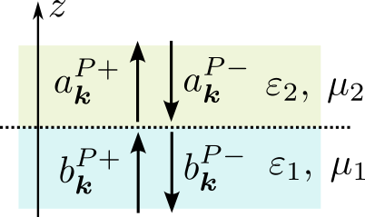
Without restriction of generality, we can put $k_y=0$ (the projection of the wavenumber/momentum of the wave in the $XY$ plane is preserved). Then the interface conditions and orthogonality of the exponential multipliers $\exp(i\boldsymbol{\varkappa}\boldsymbol{\rho})$ lead to the following equations \begin{align*} \left( b_{\boldsymbol{k}}^{s+} + b_{\boldsymbol{k}}^{s-} \right) \hat{\boldsymbol{e}}_{y} + \frac{k_{z1}}{\omega\varepsilon_{1}} \left( b_{\boldsymbol{k}}^{p+} - b_{\boldsymbol{k}}^{p-} \right) \hat{\boldsymbol{e}}_{x} &= \left( a_{\boldsymbol{k}}^{s+} + a_{\boldsymbol{k}}^{s-} \right) \hat{\boldsymbol{e}}_{y} + \frac{k_{z2}}{\omega\varepsilon_{2}} \left( a_{\boldsymbol{k}}^{p+} - a_{\boldsymbol{k}}^{p-} \right) \hat{\boldsymbol{e}}_{x} \\ \left( b_{\boldsymbol{k}}^{p+} + b_{\boldsymbol{k}}^{p-}\right) \hat{\boldsymbol{e}}_{y}-\dfrac{k_{z1}}{\omega\mu_{1}}\left(b_{\boldsymbol{k}}^{s+} - b_{\boldsymbol{k}}^{s-}\right)\hat{\boldsymbol{e}}_{x} &= \left(a_{\boldsymbol{k}}^{p+}+a_{\boldsymbol{k}}^{p-}\right) \hat{\boldsymbol{e}}_{y}-\dfrac{k_{z2}}{\omega\mu_{2}}\left(a_{\boldsymbol{k}}^{s+}-a_{\boldsymbol{k}}^{s-}\right)\hat{\boldsymbol{e}}_{x} \end{align*} from which there follows the relation between the field expansion coefficients for plane waves on both sides of the interface. This relation can be written in a form identical for both polarisations if we introduce a variable $\eta$ such that $\eta\equiv\mu$ for the ‘s’-polarization and $\eta\equiv\varepsilon$ for the ‘p’-polarization. Let us express the amplitudes of waves propagating away from the interface $a^+$, $b^-$ via the amplitudes of the waves incident on the interface $a^-$, $b^+$ (we also omit the lower index because the relations are diagonal relative to the projection of the wave vector on the plane $XY$): \begin{equation*} \left( \! \begin{array}{c} b^- \\ a^+ \end{array} \! \right) = \left( \! \begin{array}{cc} r_{11} & t_{12} \\ t_{21} & r_{22} \end{array} \! \right) \left( \! \begin{array}{c} b^+ \\ a^- \end{array} \! \right) = S \left( \! \begin{array}{c} b^+ \\ a^- \end{array} \! \right) \end{equation*} where the coefficients of the matrix $S$ are the amplitude coefficients of Fresnel reflection and transmission, and the matrix is called the scattering matrix or $S$-matrix. Explicitly \begin{align*} r_{11} &= \dfrac{\eta_{2}k_{z1}-\eta_{1}k_{z2}}{\eta_{1}k_{z2}+\eta_{2}k_{z1}} \\ t_{12} &= \dfrac{2\eta_{1}k_{z2}}{\eta_{1}k_{z2}+\eta_{2}k_{z1}} = 1-r_{11} \\ t_{21} &= \dfrac{2\eta_{2}k_{z1}}{\eta_{1}k_{z2}+\eta_{2}k_{z1}} = 1+r_{11} \\ r_{22} &= \dfrac{\eta_{1}k_{z2}-\eta_{2}k_{z1}}{\eta_{1}k_{z2}+\eta_{2}k_{z1}} = -r_{11} \end{align*} The convenience of writing these coefficients through the $z$-projections of the wavevector is that this form does not change for all possible cases of wave interation at the interface, including inhomogeneous waves and complex values of material parameters.

The relationship between the amplitudes can be written in another way, in the form of a T-matrix that relates the amplitudes on one side of the interface to the amplitudes on the other side: \begin{equation*} \left( \! \begin{array}{c} a^- \\ a^+ \end{array} \! \right) = T \left( \! \begin{array}{c} b^- \\ b^+ \end{array} \! \right) \end{equation*} Explicitly, \begin{align*} T_{11} = T_{22} &= \frac{1}{2} \left( 1+\dfrac{\eta_{1}k_{z2}}{\eta_{2}k_{z1}} \right) \\ T_{12} = T_{21} &= \frac{1}{2} \left( \dfrac{\eta_{1}k_{z2}}{\eta_{2}k_{z1}}-1 \right) \end{align*} Note that the T-matrix is also often defined through the relation between the amplitudes of the projections of the electric and magnetic fields on the $X,Y$ axes.

Reflection and transmision at a spherical boundary¶

Now let us consider the spherically symmetric case and carry out a similar derivation for spherical waves. Let us write the decomposition of an arbitrary monochromatic field through vector spherical waves in the volume of a homogeneous isotropic medium without sources as follows \begin{align*} \boldsymbol{E}(k\boldsymbol{r}) &= \sum_{m,n}\sum_{\sigma=1,3} \left[ a^{\sigma}_{mn} \boldsymbol{M}^{\sigma}_{mn}(k\boldsymbol{r}) + b^{\sigma}_{mn} \boldsymbol{N}^{\sigma}_{mn}(k\boldsymbol{r}) \right] \\ \boldsymbol{H}(k\boldsymbol{r}) = \dfrac{i}{\omega\mu} \nabla \times {\boldsymbol E}(k\boldsymbol{r}) &= \dfrac{ik}{\omega\mu} \sum_{m,n} \sum_{\sigma=1,3} \left[ b^{\sigma}_{mn} \boldsymbol{M}^{\sigma}_{mn}(k\boldsymbol{r}) + a^{\sigma}_{mn} \boldsymbol{N}^{\sigma}_{mn}(k\boldsymbol{r}) \right] \end{align*} This definition differs from the plane wave case in the sense that for both polarizations $a^{\sigma}_{mn},b^{\sigma}_{mn}$ denote the electric field amplitudes. Here it should be noted that if the region of space where the field is written in this form includes the origin (point $r=0$), then in the expansion there should be no terms with spherical waves diverging in zero, i.e., it is necessary to put $a^{3}_{mn}\equiv0$. The field in a homogeneous isotropic region of space without sources must be finite.

Let a spherical boundary $r = R$ separate two homogeneous isotropic media with material constants $\varepsilon_{1,2}$, $\mu_{1,2}$ int the vicinity of this boundary. The inner homogeneous region may or may not include the origin. Let us write the interface conditions \begin{equation*} E_{\theta,\phi}(R-0,\theta,\phi) = E_{\theta,\phi}(R+0,\theta,\phi), \; H_{\theta,\phi}(R-0,\theta,\phi) = H_{\theta,\phi}(R+0,\theta,\phi) \end{equation*} Let us substitute the explicit expression of the field components through the projections of vector spherical waves onto unit vectors of the spherical coordinate system, integrate by angular coordinates and use the orthogonality of spherical harmonics. The components corresponding to different polarizations separate. We denote the amplitudes near the boundary for $r<R$ by the upper index $(1)$, for $r>R$ by the upper index $(2)$. \begin{align*} a_{nm}^{(1)1}j_{n}\left(k_{1}R\right) - a_{nm}^{(2)3}h_{n}^{(1)}\left(k_{2}R\right) &= a_{nm}^{(2)1}j_{n}\left(k_{2}R\right) - a_{nm}^{(1)3}h_{n}^{(1)}\left(k_{1}R\right) \\ \dfrac{\mu_{2}}{\mu_{1}}a_{nm}^{(1)1}\tilde{j}_{n}\left(k_{1}R\right) - a_{nm}^{(2)3}\tilde{h}_{n}^{(1)}\left(k_{2}R\right) &= a_{nm}^{(2)1}\tilde{j}_{n}\left(k_{2}R\right) - \dfrac{\mu_{2}}{\mu_{1}}a_{nm}^{(1)3}\tilde{h}_{n}^{(1)}\left(k_{1}R\right) \\ b_{nm}^{(1)1}\tilde{j}_{n}\left(k_{1}R\right) - b_{nm}^{(2)3}\dfrac{k_{1}}{k_{2}}\tilde{h}_{n}^{(1)}\left(k_{2}R\right) &= b_{nm}^{(2)1}\dfrac{k_{1}}{k_{2}}\tilde{j}_{n}\left(k_{2}R\right) - b_{nm}^{(1)3}\tilde{h}_{n}^{(1)}\left(k_{1}R\right) \\ b_{nm}^{(1)1}\dfrac{k_{1}}{k_{2}}\dfrac{\mu_{2}}{\mu_{1}}j_{n}\left(k_{1}R\right) - b_{nm}^{(2)3}h_{n}^{(1)}\left(k_{2}R\right) &= b_{nm}^{(2)1}j_{n}\left(k_{2}R\right) - b_{nm}^{(1)3}\dfrac{k_{1}}{k_{2}}\dfrac{\mu_{2}}{\mu_{1}}h_{n}^{(1)}\left(k_{1}R\right) \end{align*} Let us write the relations between the coefficients in the form of an S-matrix. By analogy with the case of plane waves, the coefficients of this matrix can be interpreted as transmission and reflection coefficients: \begin{equation*} \left( \! \begin{array}{c} a^{(1)1}_{mn} \\ a^{(2)3}_{mn} \end{array} \! \right) = \left( \! \begin{array}{cc} r_{11mn} & t_{12mn} \\ t_{21mn} & r_{22mn} \end{array} \! \right) \left( \! \begin{array}{c} a^{(1)3}_{mn} \\ a^{(2)1}_{mn} \end{array} \! \right) = S^{P}_{mn} \left( \! \begin{array}{c} a^{(1)3}_{mn} \\ a^{(3)1}_{mn} \end{array} \! \right) \end{equation*} and similarly for the coefficients $b^{P\sigma}_{mn}$. To compute the coefficients of the matrix in explicit form, it is necessary to use the relation that follows from the Wronskian formulas for spherical Bessel functions: \begin{equation*} j_{n}(z)\frac{d}{dz}[zh_n^{(1)}(z)] - h_n^{(1)}(z)\frac{d}{dz}[zj_n(z)] = \frac{i}{z} \end{equation*} Thus, we get \begin{align*} r_{11mn} =& \dfrac{\dfrac{\mu_{2}}{\mu_{1}}h_{n}^{(1)}\left(k_{2}R\right)\tilde{h}_{n}^{(1)}\left(k_{1}R\right)-h_{n}^{(1)}\left(k_{1}R\right)\tilde{h}_{n}^{(1)}\left(k_{2}R\right)}{j_{n}\left(k_{1}R\right)\tilde{h}_{n}^{(1)}\left(k_{2}R\right)-\dfrac{\mu_{2}}{\mu_{1}}h_{n}^{(1)}\left(k_{2}R\right)\tilde{j}_{n}\left(k_{1}R\right)} \\ t_{12mn} =& \frac{i}{k_{2}R}\dfrac{1}{j_{n}\left(k_{1}R\right)\tilde{h}_{n}^{(1)}\left(k_{2}R\right)-\dfrac{\mu_{2}}{\mu_{1}}h_{n}^{(1)}\left(k_{2}R\right)\tilde{j}_{n}\left(k_{1}R\right)} \\ t_{21mn} =& \dfrac{\mu_{2}}{\mu_{1}}\frac{i}{k_{1}R}\dfrac{1}{j_{n}\left(k_{1}R\right)\tilde{h}_{n}^{(1)}\left(k_{2}R\right)-\dfrac{\mu_{2}}{\mu_{1}}h_{n}^{(1)}\left(k_{2}R\right)\tilde{j}_{n}\left(k_{1}R\right)} \\ r_{22mn} =& \dfrac{\dfrac{\mu_{2}}{\mu_{1}}j_{n}\left(k_{2}R\right)\tilde{j}_{n}\left(k_{1}R\right)-j_{n}\left(k_{1}R\right)\tilde{j}_{n}\left(k_{2}R\right)}{j_{n}\left(k_{1}R\right)\tilde{h}_{n}^{(1)}\left(k_{2}R\right)-\dfrac{\mu_{2}}{\mu_{1}}h_{n}^{(1)}\left(k_{2}R\right)\tilde{j}_{n}\left(k_{1}R\right)} \end{align*} Equations for the second polarizations are analogous.

The case of cylindrical waves can be treated similarly.

S- и Т-matrix mehtods¶

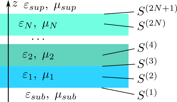
The matrices introduced above allow us to calculate propagation of waves in layered media consisting of homogeneous layers and media with spatially inhomogeneous distribution of material parameters. In the simplest case, the material parameters depend on the coordinate $z$ when using the plane wave basis or on the distance to the origin $r$ when using the spherical wave basis. Then the scattering and transmission matrices remain diagonal with respect to this basis, which greatly simplifies both the formulation of the methods and the calculations.

To formulate methods for calculating the propagation of waves, namely, when for a given external incident wave it is necessary to calculate the radiation field in the whole space, in addition to the above derived S- and T-matrices of the boundaries of medium partitions, we need appropriate matrices that allow us to relate the wave amplitudes at different spatial points of the same homogeneous isotropic medium. In the case of Cartesian coordinates, the scattering matrix of such a homogeneous layer of thickness $\ell$ should yield the phase gain of the corresponding waves due to the thickness of this layer: \begin{equation*} S_{\ell} = \left( \! \begin{array}{cc} 0 & \exp{(ik_z\ell)} \\ \exp{(ik_z\ell)} & 0 \end{array} \! \right) \end{equation*}

\begin{equation*} T_{\ell} = \left( \! \begin{array}{cc} \exp{(-ik_z\ell)} & 0 \\ 0 & \exp{(ik_z\ell)} \end{array} \! \right) \end{equation*}

In the case of spherical geometry, the S-matrix of a homogeneous spherical layer will be a matrix with units on the side diagonal and the T-matrix will be a matrix with units on the main diagonal.

The main step of the methods is the operation of composing two matrices, $S^{(1,2)}$ or $T^{(1,2)}$, for neighbouring spatial regions, such as the interface matrix and the homogeneous layer matrix. This operation allows us to obtain the matrix of a composite region from the matrices of subregions. As follows from the definition, for T-matrices such a composition is given by the usual matrix product: \begin{equation*} T = T^{(2)} T^{(1))} \end{equation*} For S-matrices, the composition $S = S^{(2)} \ast S^{(1)}$ is given by the following rule: \begin{align*} S_{11} =& S^{(1)}_{11} + S^{(1)}_{12} \left( 1-S^{(2)}_{11}S^{(1)}_{22} \right)^{-1} S^{(2)}_{11} S^{(1)}_{21} \\ S_{12} =& S^{(1)}_{12} \left( 1-S^{(2)}_{11}S^{(1)}_{22} \right)^{-1} S^{(2)}_{12} \\ S_{21} =& S^{(2)}_{21} \left( 1-S^{(1)}_{22}S^{(2)}_{11} \right)^{-1} S^{(1)}_{21} \\ S_{22} =& S^{(2)}_{22} + S^{(2)}_{21} \left( 1-S^{(1)}_{22}S^{(2)}_{11} \right)^{-1} S^{(1)}_{22} S^{(2)}_{12} \\ \end{align*} The transfer matrix method is convenient in terms of obtaining analytical results, the scattering matrix method is computationally stable.

To calculate reflection and transmission through an arbitrary inhomogeneous layer, flat, spherical or cylindrical, where the change of material parameters in the corresponding dimension is given, it is necessary to break it into a finite number of sublayers thin compared to the wavelength in the material and to consider the system as a multilayer consisting of successive homogeneous layers.

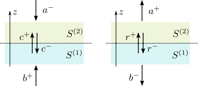
To find the field inside an inhomogeneous structure at a given coordinate, it is necessary to consider two matrices, $S^{(1,2)}$ or $T^{(1,2)}$, of substructures bordering along this coordinate, and from the given amplitudes of waves incident on the structure from external sources located outside the structure, find the amplitudes of waves inside the structure: \begin{equation*} \left( \! \begin{array}{c} c^- \\ c^+ \end{array} \! \right) = \left( \! \begin{array}{cc} \left( 1-S^{(2)}_{11}S^{(1)}_{22} \right)^{-1} S^{(2)}_{11} S^{(1)}_{21} & \left( 1-S^{(2)}_{11}S^{(1)}_{22} \right)^{-1} S^{(2)}_{12} \\ \left( 1-S^{(1)}_{22}S^{(2)}_{11} \right)^{-1} S^{(1)}_{21} & \left( 1-S^{(1)}_{22}S^{(2)}_{11} \right)^{-1} S^{(1)}_{11} S^{(2)}_{12} \end{array} \! \right) \left( \! \begin{array}{c} b^+ \\ a^- \end{array} \! \right) \end{equation*}

If a source is located inside an inhomogeneous structure, and $S^{(1,2)}$ are the matrices of substructures surrounding this source, the radiation field outside the structure can be found by the formulas \begin{equation*} \left( \! \begin{array}{c} b^- \\ a^+ \end{array} \! \right) = \left( \! \begin{array}{cc} S^{(1)}_{12} \left( 1-S^{(2)}_{11}S^{(1)}_{22} \right)^{-1} & S^{(1)}_{12} \left( 1-S^{(2)}_{11}S^{(1)}_{22} \right)^{-1} S^{(2)}_{11} \\ S^{(2)}_{21} \left( 1-S^{(1)}_{22}S^{(2)}_{11} \right)^{-1} S^{(1)}_{22} & S^{(2)}_{21} \left( 1-S^{(1)}_{22}S^{(2)}_{11} \right)^{-1} \end{array} \! \right) \left( \! \begin{array}{c} r^- \\ r^+ \end{array} \! \right) \end{equation*} where $r^{\pm}$ are the amplitudes in a homogeneous isotropic medium.

Illistration to the field calculation inside a structure (left), and calculation of the radiation field due to sources inside a structure (right)

Planar waveguide¶

Let us consider an example of a planar waveguide - a layer of homogeneous material $-h/2\leq z\leq h/2$ with dielectric constant $\varepsilon_2$, located between two semi-infinite liners with dielectric constant $\varepsilon_{1,3}$. Let us denote the reflection coefficients at the lower and upper boundary of the layer for waves incident from inside the layer as $r_L$ and $r_U$, respectively. Then the scattering matrices of the lower boundary, the waveguide material layer, and the upper boundary are as follows \begin{equation*} S^{(1)} = \left(\begin{array}{cc} -r_{L} & 1+r_{L} \\ 1-r_{L} & r_{L} \end{array}\right), \; S^{(2)} = \left(\begin{array}{cc} 0 & e^{ik_zh} \\ e^{ik_zh} & e^{ik_zh} \end{array}\right), \; S^{(3)}=\left(\begin{array}{cc} r_{U} & 1-r_{U} \\ 1+r_{U} & -r_{U} \end{array}\right) \end{equation*} Their composition gives the scattering matrix of the waveguide: \begin{equation*} S = \left(\begin{array}{cc} -r_{L} + \dfrac{r_{L}\left(1-r_{L}^{2}\right)e^{2ik_{z}h}}{1-r_{U}r_{L}e^{2ik_{z}h}} & \dfrac{\left(1+r_{L}\right)\left(1-r_{U}\right)e^{ik_{z}h}}{1-r_{U}r_{L}e^{2ik_{z}h}} \\ \dfrac{\left(1+r_{U}\right)\left(1-r_{L}\right)e^{ik_{z}h}}{1-r_{U}r_{L}e^{2ik_{z}h}} & -r_{U}+\dfrac{r_{L}\left(1-r_{U}^{2}\right)e^{2ik_{z}h}}{1-r_{U}r_{L}e^{2ik_{z}h}} \end{array}\right) \end{equation*} where $k_z$ is the projection of the wavevector inside the layer.

In applications, the considered layer can act both as a waveguiding structure and as a Fabry-Perot resonator. The scattering matrix provides a unified way to describe the layer, allowing us to obtain both discrete and continuous spectra. Suppose a field given by the amplitude vector $\boldsymbol{a}_{inc}$ is incident on the structure, and the scattered field is given by the vector $\boldsymbol{a}_{sca}$. Let us write the relation between them through the inverse matrix $S^{-1}\boldsymbol{a}_{sca} = \boldsymbol{a}_{inc}$. If the right-hand side is zero, the solutions to this equation will be the eigenvalues of $\boldsymbol{a}_{eig}$, i.e., the eigennumbers will be determined by the poles of the scattering matrix.

Let $r_U = r_L = r$ for simplicity. From the explicit form of the matrix derived above we obtain the condition: \begin{equation*} 1-r^{2}\exp\left(2ik_{z}h\right) = 0 \end{equation*} In the case of the Fabry-Perot operation mode, the wavelength is such that $|r|<1$, and by writing the condition on the phases, the Fabry-Perot resonance condition is obtained: \begin{align*} & \Re e\left\{ k_{z}\right\} h+\arg\left(r\right)=\pi l,\thinspace l\in\mathbb{Z} \\ & \exp\left(-\Im m\left\{ k_{z}\right\} h\right)=\left|r\right| \end{align*} In a purely dielectric structure, where the refractive index of the layer is higher than the refractive index of the claddings, waveguide modes can be obtained by accounting for the fact that at total internal reflection $|r|=1$, since the projection of the wave vector inside the layer $k_z$ is a real number, while outside it is a purely imaginary number $i\kappa_z = i\sqrt{k_x^2-\omega^2\varepsilon_1\mu_1}$$. For example, for the TE polarization \begin{equation*} \dfrac{\mu_{1}k_{z}-i\mu_{2}\chi_{z}}{\mu_{1}k_{z}+i\mu_{2}\chi_{z}}\exp\left(ik_{z}h\right)=\pm1 \end{equation*} Dividing this equation into real and imaginary parts, the usual dispersion equations for a plane waveguide can be obtained by simple algebraic transformations: \begin{align*} & \dfrac{\mu_{1}}{\mu_{2}}k_{z}\tan\left(\dfrac{k_{z}h}{2}\right) = \sqrt{\omega^{2}\left(\varepsilon_2\mu_2-\varepsilon_{1}\mu_{1}\right)-k_{z}^{2}} \\ & \dfrac{\mu_{1}}{\mu_{2}}k_{z}\cot\left(\dfrac{k_{z}h}{2}\right) = -\sqrt{\omega^{2}\left(\varepsilon_2\mu_2-\varepsilon_{1}\mu_{1}\right)-k_{z}^{2}} \end{align*} Their solutions have a simple graphical visualisation as intersections of the tangent and arctangent curves with the arc of a circle.

Cauchy problem for the reflection coefficient of an inhomogeneous layer¶

The calculation of propagation in an inhomogeneous one-dimensional structure can be formulated as a Cauchy problem for some differential equation. To obtain it, let us consider the obtained expression for the scattering matrix of a certain layer and set the thickness of the layer to zero. Let the problem be to determine the reflection coefficient as a function of the coordinate on the thickness of an inhomogeneous layer $r(z)$. Then the initial condition is $r(-h/2)=0$. In the equation for the scattering matrix for a thin layer of thickness $\Delta\ll n\lambda$ located at a point with coordinate $z$, let $r_L = -r(z)$, and decompose the Fresnel coefficient by the small parameter $\Delta$: \begin{equation*} r_{U}=\dfrac{k_{z}\left(z\right)/\eta\left(z\right)-k_{z}\left(z+\Delta\right)/\eta\left(z+\Delta\right)}{k_{z}\left(z+\Delta\right)/\eta\left(z+\Delta\right)+k_{z}\left(z\right)/\eta\left(z\right)}\approx-\dfrac{\left(k_{z}/\eta\right)'}{2\left(k_{z}/\eta\right)}\Delta \end{equation*} Then for the reflection coefficient given by the element $S_{22}$, \begin{equation*} r\left(z+\Delta\right)=\dfrac{-r_{U}+r\left(z\right)e^{2ik_{z}\Delta}}{1-r\left(z\right)r_{U}e^{2ik_{z}\Delta}} \approx \left(\dfrac{\left(k_{z}/\eta\right)'}{2\left(k_{z}/\eta\right)}-r^{2}\left(z\right)\dfrac{\left(k_{z}/\eta\right)'}{2\left(k_{z}/\eta\right)}+r\left(z\right)2ik_{z}\right)\Delta+r\left(z\right) \end{equation*} Hence at $\Delta\rightarrow0$ we obtain the required differential equation, which can be solved, for example, by the Runge-Kutta method: \begin{equation*} \dfrac{dr}{dz}=2ik_{z}r\left(z\right)+\dfrac{\left(k_{z}/\eta\right)'}{2\left(k_{z}/\eta\right)}\left[1-r^{2}\left(z\right)\right] \end{equation*}

References¶

Orfanidis, J. Electromagnetic waves and antennas, Ch. 5-8 Rutgers University (2016)
N. P. K. Cotter, T. W. Preist, and J. R. Sambles, Scattering-matrix approach to multilayer diffraction, J. Opt. Soc. Am. A 12, 1097-1103 (1995)
A.A. Shcherbakov, A.V. Tishchenko, D.S. Setz, B.C. Krummacher, Rigorous S-matrix approach to the modeling of the optical properties of OLEDs, Organic Electronics 12, 4, 654-659 (2011)
J. E. Davis, Multilayer reflectivity (2014)