Back to the main Index
Phonon linewidths and Eliashberg function in metals
Aluminium
In this lesson, we discuss how to compute the phonon linewidths and the Eliashberg function in metals. We start with a very brief discussion of the basic equations and some technical details about the Abinit implementation. Then we show how to build an AbiPy flow to automate the multiple steps required by these calculations.
In the second part, we use the AbiPy objects to analyze the results. We start from the simplest case of a single calculation whose most important results are stored in the A2F.nc netcdf file. Then we show how to use the A2fRobot to handle multiple netcdf files and perform convergence studies.
Table of Contents
- A bit of theory
- Technical details
- Building the Flow
- Electronic properties
- Vibrational properties
- Linewidths and Eliashberg function
- Convergence studies with A2FRobot
A bit of theory and some details about the implementation
[back to top] $\newcommand{\kk}{{\mathbf k}}$ $\newcommand{\qq}{{\mathbf q}}$ $\newcommand{\kpq}{{\kk+\qq}}$ $\newcommand{\RR}{{\mathbf R}}$ $\newcommand{\rr}{{\mathbf r}}$ $\newcommand{\<}{\langle}$ $\renewcommand{\>}{\rangle}$ $\newcommand{\KS}{{\text{KS}}}$ $\newcommand{\ww}{\omega}$ $\newcommand{\ee}{\epsilon}$ $\newcommand{\dd}{{\,\text{d}}}$
The phonon linewidths are proportional to the electron phonon coupling, and depend on the phonon wavevector $q$ and the branch index $\nu$:
\begin{equation} \gamma_{\qq\nu} = 2\pi \omega_{\qq\nu} \sum_{mn\kk} |g_{mn\nu}(\kk, \qq)|^2 \delta(\ee_{\kpq m}) \delta(\ee_{\kk n}) \end{equation}Throughout these notes we shall use Hartree atomic units ($e = \hbar = m_e = 1$), the Fermi level is set to zero.
The electron-phonon matrix elements are defined by:
\begin{equation} %\label{eq:eph_matrix_elements} g_{mn}^{\nu}(\kk,\qq) = \dfrac{1}{\sqrt{2\omega_{\qq\nu}}} \<\psi_{m \kpq} | \Delta_{\qq\nu} V^\KS |\psi_{n\kk}\> \end{equation}For further details about $\Delta_{\qq\nu} V^\KS$ and their Fourier interpolation see the previous lesson on the EPH self-energy and Phys. Rev. B 78, 045124.
The Eliashberg function, $\alpha^2F(\omega)$, is similar to the density of states of the phonons, $F(\omega)$, but is weighted according to the coupling of the phonons to the electrons:
\begin{equation} \alpha^2F(\omega) = -\dfrac{1}{N_F} \sum_{\qq\nu} \dfrac{\gamma_{\qq\nu}}{\omega_{\qq\nu}} \delta(\ww - \ww_{\qq \nu}) \end{equation}The first inverse moment of $\alpha^2F(\omega)$ gives the total coupling strength, or mass renormalization factor, $\lambda$.
\begin{equation} \lambda = \int \dfrac{\alpha^2F(\omega)}{\omega}\dd\omega = \sum_{\qq\nu} \lambda_{\qq\nu} \end{equation}\begin{equation} \lambda_{\qq\nu} = \dfrac{\gamma_{\qq\nu}}{\pi N_F \ww_{\qq\nu}^2} \end{equation}From $\lambda$, using the McMillan formula as modified by Allen and Dynes in Phys. Rev. B 12 905, one can estimate the superconducting critical temperature $T_c$ in the isotropic case.
\begin{equation} T_c = \dfrac{\omega_{log}}{1.2} \exp \Biggl [ \dfrac{-1.04 (1 + \lambda)}{\lambda ( 1 - 0.62 \mu^*) - \mu^*} \Biggr ] \end{equation}where the logarithmic moment, $\omega_{log}$, is defined by:
\begin{equation} \omega_{log} = \exp \Biggl [ \dfrac{2}{\lambda} \int \dfrac{\alpha^2F(\omega)}{\omega}\log(\omega)\dd\omega \Biggr ] \end{equation}The formula contains the $\mu^*$ parameter which approximates the effect of the Coulomb interaction. It is common to treat $\mu^*$ as an adjustable parameter to reproduce (explain) the experimental $T_c$ from the ab-initio computed $\lambda$.
It is worth noting that, if we assume constant e-ph matrix elements in the BZ, the phonon linewidths become proportional to the so-called nesting function defined by:
\begin{equation} N(\qq) = \sum_{mn\kk} \delta(\ee_{\kpq m}) \delta(\ee_{\kk n}) \end{equation}Roughly speaking, there are two factors entering into play in the equation for the phonon linewidths: the behaviour in (k, q) space of the matrix elements and the geometrical contribution related to the shape of the Fermi surface (described by the nesting term).
Implementation details:
The input variables optdriver = 7 and eph_task = 1 activate the computation of:
\begin{equation} \gamma_{\qq\nu} = 2\pi \omega_{\qq\nu} \sum_{pp'} d_{\qq p}^* \tilde\gamma_{p p'}(\qq) d_{\qq p'}^* \end{equation}for all q-points in the IBZ as determined by the ddb_ngqpt input variable.
In the above equation, $p$ is a short-hand notation for atom index and direction,
$\vec d$ is the phonon displacement and $\tilde\gamma_{p p'}(\qq)$ is given by:
The $\tilde\gamma_{p p'}(\qq)$ matrix has the same symmetries as the dynamical matrix and the elements in the full BZ can be obtained by rotating the initial set of q-points in the IBZ.
Once $\tilde\gamma(\qq)$ is known in the full BZ, one can Fourier transform to real space with:
\begin{equation} \tilde\gamma_{p p'}(\RR) = \sum_\qq e^{i\qq\cdot\RR} \tilde\gamma_{p p'}(\qq) \end{equation}and use Fourier interpolation to obtain $\gamma_{\qq\nu}$ everywhere in the BZ at low cost (a similar approach is used for the dynamical matrix and phonon frequencies).
Thanks to the relatively inexpensive Fourier interpolation, one can obtain the phonon linewidths along
an arbitrary q-path and evaluate the Eliashberg function on a q-mesh (specified by ph_ngqpt)
that can be made much denser than the initial ab-initio DDB sampling (specified by ddb_ngqpt) and
even denser than the eph_ngqpt_fine q-mesh used to interpolate the DFPT potentials.
Note that the calculation of phonon linewidths in metals is made difficult
by the slow convergence of the double-delta integral over the Fermi surface.
It is therefore convenient to use a coarse k-mesh to calculate phonons with DFPT on a suitable q-grid
and then use a denser k-mesh to perform the integration over the Fermi surface.
The resolution in q-space can be improved by interpolating the DFPT potentials via the
eph_ngqpt_fine input variable as discussed in the previous EPH lesson.
Suggested references
The general theory of electron-phonon coupling and Eliashberg superconductivity is reviewed by P.B. Allen and B. Mitrovic in Theory of Superconducting Tc. The first implementations similar to that in Abinit are those in Savrasov and Liu.
Technical details
From the previous discussion, it should be clear that a typical calculation of phonon linewidths requires:
- An initial set of KS wavefunctions and eigenvalues.
- The knowledge of the dynamical matrix $D(\qq)$ from which one can obtain frequencies and displacements everywhere in the BZ via Fourier interpolation.
- A set of DFPT potentials given in the IBZ
Thanks to these three ingredients, the code can compute the EPH matrix elements and perform the integration over the Fermi surface. A schematic representation of a typical workflow with Abinit is given in the figure below:
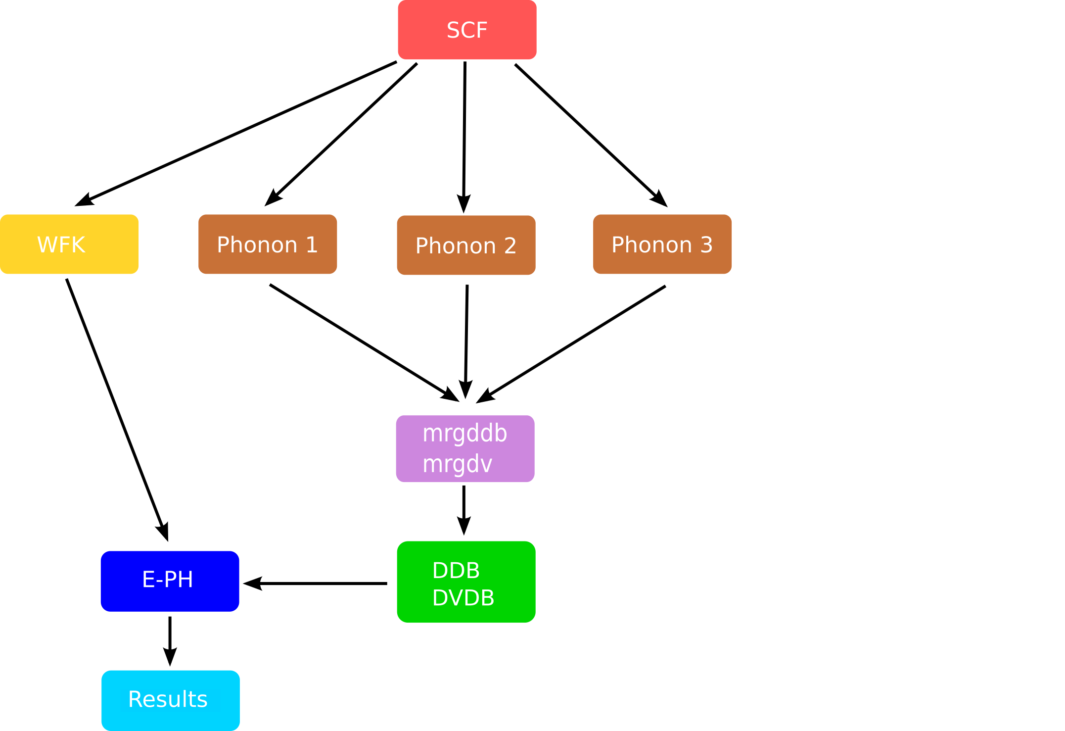
The mrgddb and mrgdv are Fortran executables whose main goal is to produce the final files
required in the EPH code.
Note, in particular, how the computation of the WFK file and the DFPT part of the graph are now decoupled. This is the approach we are going to implement with AbiPy to converge the phonon linewidths in Al:
Compute DFPT phonons on a 4x4x4 q-mesh with a coarse 8x8x8 k-sampling
Generate 3 WFK files on a much denser k-mesh (x16, x24, x32)
Run the EPH code with
- one of the WFK files generated in point 2.
- interpolated DFPT potentials (from the initial 4x4x4 to a 8x8x8 q-mesh)
- Compute the Eliashberg function on the
ph_ngqptmesh via Fourier interpolation. - Analyze the convergence of the results wrt
nkpt.
Building the Flow
Before starting, we need to import the python modules used in this notebook:
# Use this at the beginning of your script so that your code will be compatible with python3
from __future__ import print_function, division, unicode_literals

import numpy as np
import warnings
warnings.filterwarnings("ignore") # to get rid of deprecation warnings

from abipy import abilab
abilab.enable_notebook() # This line tells AbiPy we are running inside a notebook
import abipy.flowtk as flowtk

# This line configures matplotlib to show figures embedded in the notebook.
# Replace `inline` with `notebook` in classic notebook
%matplotlib inline

# Option available in jupyterlab. See https://github.com/matplotlib/jupyter-matplotlib
#%matplotlib widget
and a function from the lesson_eph_al module to build our AbiPy flow.
from lesson_eph_al import build_flow
abilab.print_source(build_flow)
def build_flow(options):
    """
    Build and return an AbiPy flow to compute phonon linewidths and Eliashberg function in Aluminium:

        1. Compute DFPT phonons on a 4x4x4 q-mesh with a coarse 8x8x8 k-sampling

        2. Generate 3 WFK files on a much denser k-mesh (x16, x24, x32)

        3. Run the EPH code with:

          - one of the WFK files generated in point 2.
          - interpolated DFPT potentials (from the initial 4x4x4 to a 8x8x8 q-mesh)

        4. Analyze the convergence of the results wrt nkpt.

    Note that the q-point grid must be a sub-grid of the k-point grid
    """
    workdir = options.workdir if (options and options.workdir) else "flow_eph_al"

    # Create empty flow.
    flow = flowtk.Flow(workdir=workdir)

    # Init structure. Use NC pseudo
    structure = abilab.Structure.fcc(a=7.5, species=["Al"], units="bohr")
    pseudos = abidata.pseudos("Al.oncvpsp")

    # Input for GS part.
    gs_inp = abilab.AbinitInput(structure, pseudos)
    gs_inp.set_vars(
        istwfk="*1",
        ecut=8.0,
        nband=4,
        occopt=7,      # Include metallic occupation function with a small smearing
        tsmear=0.04,
        tolvrs=1e-7,
    )

    # The k-grid is minimalistic to keep the calculation manageable.
    gs_inp.set_kmesh(
        ngkpt=[8, 8, 8],
        shiftk=[0.0, 0.0, 0.0],
    )

    # Build new input for NSCF calculation along k-path (automatically selected by AbiPy)
    # Used to plot the KS band structure.
    nscf_kpath_inp = gs_inp.new_with_vars(
        nband=4,
        tolwfr=1e-16,
        iscf=-2,
    )
    nscf_kpath_inp.set_kpath(ndivsm=10)

    # Build NSCF inputs with denser k-meshes
    # This step generates the WFK files used to compute the Eliashberg function.
    # We have a cubic material so we only need to specify the first number of divisions.
    nk_list = [16, 24, 32]

    nscf_kmesh_inputs = []
    for nk in nk_list:
        new_inp = gs_inp.new_with_vars(
            tolwfr=1e-16,
            iscf=-2,
            ngkpt=[nk] * 3,
            shiftk=[0.0, 0.0, 0.0],
        )
        nscf_kmesh_inputs.append(new_inp)

    # Register GS + NSCF kpath + NSCF with k-meshes in work0.
    work0 = flowtk.BandStructureWork(gs_inp, nscf_kpath_inp, dos_inputs=nscf_kmesh_inputs)
    flow.register_work(work0)

    # Generate Phonon work with 4x4x4 q-mesh
    # Reuse the variables from GS input and let AbiPy handle the generation of the input files
    # Note that the q-point grid is a sub-grid of the k-mesh so we do not need WFQ on k+q mesh.
    ddb_ngqpt = [4, 4, 4]
    ph_work = flowtk.PhononWork.from_scf_task(work0[0], ddb_ngqpt, is_ngqpt=True)
    flow.register_work(ph_work)

    # Ssction for EPH calculation: compute linewidths with different WKK files.
    eph_work = flowtk.Work()
    for ik, nk in enumerate(nk_list):
        # Each task uses a different WFK file. DDB and DBDB do not change.
        eph_deps = {work0[2 + ik]: "WFK", ph_work: ["DDB", "DVDB"]}

        # Interpolate DFPT potentials 4x4x4 --> 8x8x8
        eph_ngqpt_fine = (8, 8, 8)

        # Build input for E-PH run. See also v7/Input/t85.in
        # The k-points must be in the WFK file
        eph_inp = gs_inp.new_with_vars(
            optdriver=7,                    # Enter EPH driver.
            eph_task=1,                     # Compute phonon linewidths in metals.
            ddb_ngqpt=ddb_ngqpt,            # q-mesh used to produce the DDB file (must be consistent with DDB data)
            eph_fsewin="0.8 eV",            # Energy window around Ef (only states in this window are included)
            eph_intmeth=2,                  # Tetra method
            #eph_intmeth=1,                 # Gaussian
            #eph_fsmear=eph_fsmear * abilab.units.eV_to_Ha, # Broadening
            eph_ngqpt_fine=eph_ngqpt_fine,  # Interpolate DFPT potentials if != ddb_ngqpt
            eph_mustar=0.12,                # mustar parameter
            ngkpt=[nk] * 3,
            shiftk=[0.0, 0.0, 0.0],
        )

        # Set q-path to interpolate phonons and phonon linewidths.
        eph_inp.set_qpath(10)

        # Set q-mesh for phonons DOS and a2F(w)
        eph_inp.set_phdos_qmesh(nqsmall=24, method="tetra")
        eph_work.register_eph_task(eph_inp, deps=eph_deps)

    flow.register_work(eph_work)

    # Avoid producing (big) output files that not required by children.
    flow.allocate(use_smartio=True)

    return flow
OK the function is a little bit long but it is normal as we are computing in a single workflow the electronic properties, the vibrational spectrum and the phonon linewidths with different k-point samplings.
Note that we have already encountered similar flows in the previous AbiPy lessons.
The calculation of electronic band structures is
discussed in
lesson_base3
while an example of Flow for phonon calculations is given in
lesson_dfpt.
The novelty is represented by the generation of the EphTasks
in which we have to specify several variables related to phonons and the EPH self-energy.
For your convenience, we have grouped the variables used in the EphTask in sub-groups:

Hopefully things will become clearer if we build the flow and start to play with it:
flow = build_flow(options=None)
flow.show_info()
<Flow, node_id=345822, workdir=flow_eph_al>
Number of works: 3, total number of tasks: 22
Number of tasks with a given class:

Task Class      Number
------------  --------
ScfTask              1
NscfTask             4
PhononTask          14
EphTask              3
We then print the input of the last EphTask.
Please read carefully the documentation of the variables, in particular
those in the dfpt and eph sections.
In a nutshell: we read a WKF on a 32x32x32 k-mesh and a DDB on a 4x4x4 q-mesh,
activate the computation of phonon linewidths with optdriver and eph_task,
interpolate the potentials onto a 8x8x8 q-mesh with eph_ngqpt_fine and set other variables
for the computation of the phonon linewidths around the Fermi surface.
print(flow[-1][-1])
flow[-1][-1].input
<EphTask, node_id=345856, workdir=flow_eph_al/w2/t2>
# SECTION: basic
############################################################################################
ecut 8.0
nband 4
occopt 7
tolvrs 1e-07
ngkpt 32 32 32
kptopt 1
nshiftk 1
shiftk 0.0 0.0 0.0
############################################################################################
# SECTION: dev
############################################################################################
istwfk *1
############################################################################################
# SECTION: eph
############################################################################################
eph_task 1
ddb_ngqpt 4 4 4
eph_fsewin 0.8 eV
eph_intmeth 2
eph_ngqpt_fine 8 8 8
eph_mustar 0.12
ph_ndivsm 10
ph_nqpath 12
ph_qpath
0.0 0.0 0.0
0.5 0.0 0.5
0.5 0.25 0.75
0.375 0.375 0.75
0.0 0.0 0.0
0.5 0.5 0.5
0.625 0.25 0.625
0.5 0.25 0.75
0.5 0.5 0.5
0.375 0.375 0.75
0.625 0.25 0.625
0.5 0.0 0.5
ph_intmeth 2
ph_wstep 0.0001 eV
ph_ngqpt 24 24 24
ph_qshift 0 0 0
ph_nqshift 1
############################################################################################
# SECTION: files
############################################################################################
prtwf -1
prtden 0
############################################################################################
# SECTION: gstate
############################################################################################
tsmear 0.04
optdriver 7
############################################################################################
# STRUCTURE
############################################################################################
natom 1
ntypat 1
typat 1
znucl 13
xred 0.0000000000 0.0000000000 0.0000000000
acell 1.0 1.0 1.0
rprim
0.0000000000 3.7500000000 3.7500000000
3.7500000000 0.0000000000 3.7500000000
3.7500000000 3.7500000000 0.0000000000
As usual, it is much easier to understand what is happening if we plot a graph with the individual tasks and their connections. Since there are several nodes in our graph, we mainly focus on the EPH part.
Let's have a look at the parents of the last EphTask with:
flow[-1][-1].get_graphviz()
We do not repeat here the detailed description of the Flow because it is very similar in spirit to what has been already done in the previous EPH lesson. Hopefully, you are already familiar with the AbiPy philosophy.
print("ngkpt in EPH tasks:", [task.input["ngkpt"] for task in flow[2]])
ngkpt in EPH tasks: [[16, 16, 16], [24, 24, 24], [32, 32, 32]]
flow[2].get_vars_dataframe("ngkpt")
| ngkpt | class | |
|---|---|---|
| w2_t0 | [16, 16, 16] | EphTask |
| w2_t1 | [24, 24, 24] | EphTask |
| w2_t2 | [32, 32, 32] | EphTask |
For completeness, we show the entire flow with the different connections:
flow.get_graphviz()
Now we can generate the directories and the input files of the Flow with:
flow.build_and_pickle_dump()
and then use the abirun.py script to launch the entire calculation:
abirun.py flow_eph_al scheduler
You may want to run this example in the terminal if you've already installed and configured AbiPy and Abinit on your machine. The calculation requires ~12 minutes on a poor 1.7 GHz Intel Core i5 (50% of the time is spent in the last task to compute the phonon linewidths with the 32x32x32 k-mesh)
If you prefer to skip this part, jump to next section in which we focus on the post-processing of the results. Note that most of the output files are already available in the github repository so it is possible to try the AbiPy post-processing tools without having to run the flow. Some DVDB, DDB, PHDOS, and PBSTS files are missing, but their absence will not prevent running the present tutorial to the end. In particular, one can use the command line and the commands:
abiopen.py FILE
to open the file inside ipython,
abiopen.py ut_A2F.nc --expose
to visualize the EPH results and finally,
abicomp.py a2f flow_ep_al/
to compare multiple A2F.nc files with the robot and ipython.
!find flow_eph_al/ -name "out_GSR.nc"
flow_eph_al//w0/t0/outdata/out_GSR.nc
flow_eph_al//w0/t1/outdata/out_GSR.nc
flow_eph_al//w0/t2/outdata/out_GSR.nc
flow_eph_al//w0/t3/outdata/out_GSR.nc
flow_eph_al//w0/t4/outdata/out_GSR.nc
The task w0/t0 computed the electronic band structure on a high-symmetry k-path.
Let's plot the bands with:
with abilab.abiopen("flow_eph_al/w0/t1/outdata/out_GSR.nc") as gsr:
    ebands_kpath = gsr.ebands

# NB: Fermi level set to zero
ebands_kpath.plot();

#print(ebands_kpath)
To better understand what’s happening at $\ee_F$, we can plot the bandwidths with:
ebands_kpath.boxplot();

There is only one band index crossing the Fermi level if we exclude a tiny portion with band index 2 (see the region close to the W point). As phonon lifetimes are very sensitive to the Fermi surface sampling, it is a good idea to analyze the convergence of the electronic DOS, in particular the behavior in the region around $\ee_F$.
Let's use the GsrRobot to load all the GSR files produced by the w0 work:
gsr_robot = abilab.GsrRobot.from_dir_glob("flow_eph_al/w0/t*/")
gsr_robot
- flow_eph_al/w0/t0/outdata/out_GSR.nc
- flow_eph_al/w0/t1/outdata/out_GSR.nc
- flow_eph_al/w0/t2/outdata/out_GSR.nc
- flow_eph_al/w0/t3/outdata/out_GSR.nc
- flow_eph_al/w0/t4/outdata/out_GSR.nc
In total, we have 5 GSR files but w0/t1 computed the energies along the k-path and the
DOS requires a homogeneous sampling.
Let's remove the file for which this is not the case from the robot with:
gsr_robot.pop_label("flow_eph_al/w0/t1/outdata/out_GSR.nc")
gsr_robot
- flow_eph_al/w0/t0/outdata/out_GSR.nc
- flow_eph_al/w0/t2/outdata/out_GSR.nc
- flow_eph_al/w0/t3/outdata/out_GSR.nc
- flow_eph_al/w0/t4/outdata/out_GSR.nc
and use a small lambda function to change the labels associated to the files so that we have the number of k-points in the IBZ:
gsr_robot.remap_labels(lambda gsr: "nkpt: %d" % gsr.nkpt)
OrderedDict([('nkpt: 29', 'flow_eph_al/w0/t0/outdata/out_GSR.nc'),
             ('nkpt: 145', 'flow_eph_al/w0/t2/outdata/out_GSR.nc'),
             ('nkpt: 413', 'flow_eph_al/w0/t3/outdata/out_GSR.nc'),
             ('nkpt: 897', 'flow_eph_al/w0/t4/outdata/out_GSR.nc')])
Now we can finally compare the electronic DOS obtained with the different k-meshes:
gsr_robot.combiplot_edos(xlims=[-15, +5]);

Clearly, the 8x8x8 k-mesh used to compute the density is not enough to converge the DOS at $\ee_F$. Remember, however, that we have decided to use a minimalistic sampling in the GS/DFPT run to keep the calculation manageable. In real life, one should use a much denser k-sampling for the GS/DFPT and this is particularly true if we are trying to relax the structure. Let's forget about this technical point and focus on the DOS obtained with the other two k-meshes.
As you can see, even if 145 k-points in the IBZ are not enough, the DOS is becoming smoother and starts to resemble the one of the free-electron gas (as a matter of fact the band dispersion of Al is not that different from the ideal free-electron model provided that BZ folding is taken into account).
Visual inspection suggests that the k-sampling becomes acceptable at and beyond 24x24x24 (413 nkpt).
In the introduction, we mentioned that there are two factors governing the strengh of the E-PH coupling in metals: the behaviour in (k, q)-space of the matrix elements and the geometrical contribution due to the Fermi surface.
\begin{equation} N(\qq) = \sum_{mn\kk} \delta(\ee_{\kpq m}) \delta(\ee_{\kk n}) \end{equation}To understand the geometrical contribution, it is useful to visualize the Fermi surface. Unfortunately, graphical applications usually require KS eigenvalues on a $\Gamma-$centered k-mesh in the full BZ whereas ab-initio codes usually work with KS states in the irreducible wedge.
Fortunately, we can use AbiPy to reconstruct the KS eigenvalues in the full BZ:
# Select the last GSR file in thr robot.
eb3d = gsr_robot.abifiles[-1].ebands.get_ebands3d()
and then use matplotlib to visualize the Fermi energy isosurfaces:
eb3d.plot_isosurfaces();

Note that, at present, the matplotlib version is only able to display isosurfaces in the unit cell of the reciprocal lattice. To visualize isosurfaces in the first BZ, one can export the data into BXSF format and then call xcrysden with:
#eb3d.xcrysden_view()
This is the image you should get with xcrysden:

Vibrational properties
Now we turn our attention to the vibrational properties.
AbiPy has already merged all the independent atomic perturbations in flow_eph_al/w1/outdata/out_DDB:
!find flow_eph_al/ -name "out_DDB"
flow_eph_al//w0/t0/outdata/out_DDB
flow_eph_al//w1/outdata/out_DDB
!cat flow_eph_al/w1/outdata/mrgddb.stdin
/Users/gmatteo/git_repos/abitutorials/abitutorials/eph_al/flow_eph_al/w1/outdata/out_DDB
DDB file merged by PhononWork on Sun Mar 18 14:41:09 2018
14
/Users/gmatteo/git_repos/abitutorials/abitutorials/eph_al/flow_eph_al/w1/t0/outdata/out_DDB
/Users/gmatteo/git_repos/abitutorials/abitutorials/eph_al/flow_eph_al/w1/t1/outdata/out_DDB
/Users/gmatteo/git_repos/abitutorials/abitutorials/eph_al/flow_eph_al/w1/t2/outdata/out_DDB
/Users/gmatteo/git_repos/abitutorials/abitutorials/eph_al/flow_eph_al/w1/t3/outdata/out_DDB
/Users/gmatteo/git_repos/abitutorials/abitutorials/eph_al/flow_eph_al/w1/t4/outdata/out_DDB
/Users/gmatteo/git_repos/abitutorials/abitutorials/eph_al/flow_eph_al/w1/t5/outdata/out_DDB
/Users/gmatteo/git_repos/abitutorials/abitutorials/eph_al/flow_eph_al/w1/t6/outdata/out_DDB
/Users/gmatteo/git_repos/abitutorials/abitutorials/eph_al/flow_eph_al/w1/t7/outdata/out_DDB
/Users/gmatteo/git_repos/abitutorials/abitutorials/eph_al/flow_eph_al/w1/t8/outdata/out_DDB
/Users/gmatteo/git_repos/abitutorials/abitutorials/eph_al/flow_eph_al/w1/t9/outdata/out_DDB
/Users/gmatteo/git_repos/abitutorials/abitutorials/eph_al/flow_eph_al/w1/t10/outdata/out_DDB
/Users/gmatteo/git_repos/abitutorials/abitutorials/eph_al/flow_eph_al/w1/t11/outdata/out_DDB
/Users/gmatteo/git_repos/abitutorials/abitutorials/eph_al/flow_eph_al/w1/t12/outdata/out_DDB
/Users/gmatteo/git_repos/abitutorials/abitutorials/eph_al/flow_eph_al/w1/t13/outdata/out_DDB
In the same directory, we have the DVDB file containing the independent DFPT potentials
!find flow_eph_al/ -name "out_DVDB"
flow_eph_al//w1/outdata/out_DVDB
#!cat flow_eph_al//w1/outdata/mrgdvdb.stdin
Let's open the DDB file computed on the 4x4x4 q-mesh with:
ddb = abilab.abiopen("flow_eph_al/w1/outdata/out_DDB")
print(ddb)
================================= File Info =================================
Name: out_DDB
Directory: /Users/gmatteo/git_repos/abitutorials/abitutorials/eph_al/flow_eph_al/w1/outdata
Size: 42.10 kb
Access Time: Mon Aug 13 15:11:37 2018
Modification Time: Sun Mar 18 14:41:09 2018
Change Time: Sun Mar 18 14:41:09 2018

================================= Structure =================================
Full Formula (Al1)
Reduced Formula: Al
abc   :   2.806386   2.806386   2.806386
angles:  60.000000  60.000000  60.000000
Sites (1)
  #  SP      a    b    c
---  ----  ---  ---  ---
  0  Al      0    0    0

Abinit Spacegroup: spgid: 0, num_spatial_symmetries: 48, has_timerev: True, symmorphic: False

================================== DDB Info ==================================

Number of q-points in DDB: 8
guessed_ngqpt: [4 4 4] (guess for the q-mesh divisions made by AbiPy)
Has total energy: False, Has forces: False
Has stress tensor: False

Has (at least one) atomic pertubation: True
Has (at least one diagonal) electric-field perturbation: False
Has (at least one) Born effective charge: True
Has (all) strain terms: False
Has (all) internal strain terms: False
Has (all) piezoelectric terms: False
and then invoke anaddb to compute phonon bands and DOS:
phbst, phdos = ddb.anaget_phbst_and_phdos_files()
Finally we plot the results with:
phbst.phbands.plot_with_phdos(phdos);

The vibrational spectrum seems OK but remember that we are enforcing the acoustic sum rule
with asr.
Since our input parameters are underconverged, its a good idea to compare the spectrum with/without asr:
ph_plotter = ddb.anacompare_asr()
ph_plotter.combiplot(units="cm-1");

We can now finally turn our attention to the phonon linewidths and the Eliashberg function.
Phonon linewidths and Eliashberg function
We have generated a pair of DDB-DVDB files on a 4x4x4 q-mesh
and three WFK files with a much denser k-sampling (x16, x24, x32).
In total we have three EPH calculations done with different k-meshes to analyze.
Let's focus on the output files produced with the 16x16x16 k-mesh by the first EphTask in w2/t0:
!ls flow_eph_al/w2/t0/outdata
out_A2F.nc               out_NOINTP_A2FW          out_PHDOS.nc
out_A2FW                 out_NOINTP_PH_A2FW       out_PHDOS_by_atom
out_A2FW_QPTOPT3_A2FW    out_OUT.nc               out_PHDOS_msqd
out_A2FW_QPTOPT3_PH_A2FW out_PHBANDS.agr          out_PHGAMMA
out_EBANDS.agr           out_PHBST.nc             out_PH_A2FW
out_EDOS                 out_PHDOS                out_THERMO
The most important results are stored in:
- out_A2F.nc: main results in netcdf format
- out_PHDOS.nc: phonon DOS and projections over atoms and directions
- out_PBSTS.nc: phonon band structure along the q-path
Let's get a quick summary of the most important results with:
a2fnc = abilab.abiopen("flow_eph_al/w2/t0/outdata/out_A2F.nc")
print(a2fnc)
================================= File Info =================================
Name: out_A2F.nc
Directory: /Users/gmatteo/git_repos/abitutorials/abitutorials/eph_al/flow_eph_al/w2/t0/outdata
Size: 254.68 kb
Access Time: Mon Aug 13 15:11:59 2018
Modification Time: Sun Mar 18 14:42:28 2018
Change Time: Sun Mar 18 14:42:28 2018

================================= Structure =================================
Full Formula (Al1)
Reduced Formula: Al
abc   :   2.806386   2.806386   2.806386
angles:  60.000000  60.000000  60.000000
Sites (1)
  #  SP      a    b    c
---  ----  ---  ---  ---
  0  Al      0    0    0

Abinit Spacegroup: spgid: 0, num_spatial_symmetries: 48, has_timerev: True, symmorphic: False

============================== Electronic Bands ==============================
Number of electrons: 3.0, Fermi level: 7.166 (eV)
nsppol: 1, nkpt: 145, mband: 4, nspinor: 1, nspden: 1
smearing scheme: gaussian, tsmear_eV: 1.088, occopt: 7

================================ Phonon Bands ================================
Number of q-points: 198
Atomic mass units: {13.0: 26.981539}
Has non-analytical contribution for q --> 0: False

============================== E-PH calculation ==============================
K-mesh for electrons:
mpdivs: [16 16 16] with shifts [[0. 0. 0.]] and kptopt: 1

a2f(w) on the [8 8 8] q-mesh (ddb_ngqpt|eph_ngqpt)
Isotropic lambda: 0.25, omega_log: 0.030 (eV), 343.094 (K)

a2f(w) Fourier interpolated on the [24 24 24] q-mesh (ph_ngqpt)
Isotropic lambda: 0.26, omega_log: 0.027 (eV), 314.268 (K)
In the E-PH calculation we have the value of $\lambda$ and $\omega_{log}$ computed
with a 16x16x16 k-mesh for electrons and two q-meshes.
...
The value of $\lambda$ is smaller (almost a factor 2) with respect to other values reported in the literature, likely due to the coarse 12x12x12 k-sampling. We will investigate this problem in the next section. For the time being, we prefer to focus on the visualization of the results with AbiPy.
Let's use matplotlib to plot the Eliashberg function obtained with the two q-meshes:
a2fnc.plot_a2f_interpol();

This Eliashberg function obtained on the [24, 24, 24] q-mesh looks nicer, in particular we see the appearance of Van Hove singularities. As expected, the integral $\lambda(\omega)$ is less sensitive to the interpolation in q-space. We conclude that the fact that our $\lambda$ is too small when compared with other ab-initio calculations ($\lambda \approx 0.4$) is not related to the q-sampling but to the quality of our phonon linewidths that in turn is related to the description of the FS.
We can also visualize the phonon linewidths with a scatter plot:
a2fnc.plot_with_a2f(units="meV", what="gamma");
#a2fnc.plot(units="meV", what="gamma");

To plot the band energies used in the calculation:
#a2fnc.plot_ebands();
The notation $\alpha^2 F(\omega)$ was introduced because the Eliashberg function is usually proportional to the phonon DOS $F(\omega)$. There are, however, exceptions so it is useful to plot $\alpha^2F(\omega)$, $F(\omega)$ and their ratio $\alpha^2$.
It is just a matter of passing the phonon DOS computed from the DDB file in the previous section
to the plot_a2 method:
a2fnc.a2f_qcoarse.plot_a2(phdos=phdos);

To conclude this section: our results for $\lambda$ and $\alpha^2F(\omega)$ look reasonable but we are still far from the results reported in previous works. Perhaps we are not completely converged and we should analyze in more detail what happens if we increase the k-point sampling. Fortunately we have already computed these results in our Flow so it is just a matter of using AbiPy to compare multiple calculations.
Using the A2FRobot for convergence studies
In this section, we use the A2fRobot to analyze the convergence behaviour of our results
with respect to the k-point sampling in the double-delta integral.
Let's ask our robot to open all the A2F files located within the flow_eph_al/ directory.
robot = abilab.A2fRobot.from_dir("flow_eph_al/")
robot
- w2/t0/outdata/out_A2F.nc
- w2/t1/outdata/out_A2F.nc
- w2/t2/outdata/out_A2F.nc
We know that all these calculations have been done with different values of nkpt.
Let's change the labels of the files by replacing file paths with more informative strings:
robot.remap_labels(lambda ncfile: "nkpt: %d" % ncfile.nkpt)
OrderedDict([('nkpt: 145', 'w2/t0/outdata/out_A2F.nc'),
             ('nkpt: 413', 'w2/t1/outdata/out_A2F.nc'),
             ('nkpt: 897', 'w2/t2/outdata/out_A2F.nc')])
and print a pandas DataFrame with the parameters of the calculation can help to understand the data:
robot.get_params_dataframe()
| nsppol | nspinor | nspden | nband | nkpt | ddb_nqbz | eph_nqbz_fine | ph_nqbz | eph_intmeth | eph_fsewin | eph_fsmear | eph_extrael | eph_fermie | |
|---|---|---|---|---|---|---|---|---|---|---|---|---|---|
| nkpt: 145 | 1 | 1 | 1 | 4 | 145 | 64 | 512 | 13824 | 2 | 0.029399 | 0.01 | 0.0 | 0.0 |
| nkpt: 413 | 1 | 1 | 1 | 4 | 413 | 64 | 512 | 13824 | 2 | 0.029399 | 0.01 | 0.0 | 0.0 |
| nkpt: 897 | 1 | 1 | 1 | 4 | 897 | 64 | 512 | 13824 | 2 | 0.029399 | 0.01 | 0.0 | 0.0 |
As usual, it is much easier to analyze the convergence of scalar quantities. Since we are mainly interested in $T_c$-related properties, it makes sense to print a table with the value of $\lambda$ and $\omega_{log}$ extracted from the different calculations:
robot.get_dataframe(with_params=False)
| lambda_qcoarse | omegalog_qcoarse | lambda_qintp | omegalog_qintp | |
|---|---|---|---|---|
| nkpt: 145 | 0.248242 | 0.029566 | 0.262111 | 0.027082 |
| nkpt: 413 | 0.373353 | 0.029148 | 0.401513 | 0.025940 |
| nkpt: 897 | 0.386603 | 0.028770 | 0.417210 | 0.025479 |
This table gives the values integrated on the eph_ngqpt mesh as well as the values obtained
by Fourier interpolating the results on the ph_ngqpt mesh.
Note the big jump in $\lambda$ when we go from the 18x18x18 k-mesh to the 36x36x36 k-mesh (~0.2 --> ~0.4).
This clearly shows that our initial estimate for $\lambda$ obtained with a 18x18x18 k-mesh was really bad!
(Did I tell you that these calculations are very sensitive to the k-point sampling?)
If you prefer figures instead of tables with numbers, just use:
robot.plot_a2fdata_convergence(sortby="nkpt");

When converging with respect to the number of k-points, it is common to plot the physical results as function of $\frac{1}{N_{kpt}}$. Let's define a small function that tells our robot how to sort the results:
def inv_nkpt(a2f_file):
    """$\dfrac{1}{N_k}$"""
    return 1/ a2f_file.nkpt

robot.plot_a2fdata_convergence(sortby=inv_nkpt); #, hue="eph_fsmear");

At this point, our estimate for $\lambda$ should be somewhere in [0.39, 0.42] that compares much better with the value of 0.44 reported by Savrasov. Most importantly, our results started to converge (although slowly). Now we know that a serious calculation of the phonon linewidths of Al would require something around 32x32x32 k-points (this is indeed the mesh used by Savrasov in their paper).
So far, we have been focusing on $\lambda$ but what about the convergence of $\alpha^2F(\omega)$?
robot.plot_a2f_convergence();

print(robot.abifiles[-1])
================================= File Info =================================
Name: out_A2F.nc
Directory: /Users/gmatteo/git_repos/abitutorials/abitutorials/eph_al/flow_eph_al/w2/t2/outdata
Size: 331.68 kb
Access Time: Mon Aug 13 15:12:05 2018
Modification Time: Sun Mar 18 14:49:37 2018
Change Time: Sun Mar 18 14:49:37 2018

================================= Structure =================================
Full Formula (Al1)
Reduced Formula: Al
abc   :   2.806386   2.806386   2.806386
angles:  60.000000  60.000000  60.000000
Sites (1)
  #  SP      a    b    c
---  ----  ---  ---  ---
  0  Al      0    0    0

Abinit Spacegroup: spgid: 0, num_spatial_symmetries: 48, has_timerev: True, symmorphic: False

============================== Electronic Bands ==============================
Number of electrons: 3.0, Fermi level: 7.166 (eV)
nsppol: 1, nkpt: 897, mband: 4, nspinor: 1, nspden: 1
smearing scheme: gaussian, tsmear_eV: 1.088, occopt: 7

================================ Phonon Bands ================================
Number of q-points: 198
Atomic mass units: {13.0: 26.981539}
Has non-analytical contribution for q --> 0: False

============================== E-PH calculation ==============================
K-mesh for electrons:
mpdivs: [32 32 32] with shifts [[0. 0. 0.]] and kptopt: 1

a2f(w) on the [8 8 8] q-mesh (ddb_ngqpt|eph_ngqpt)
Isotropic lambda: 0.39, omega_log: 0.029 (eV), 333.858 (K)

a2f(w) Fourier interpolated on the [24 24 24] q-mesh (ph_ngqpt)
Isotropic lambda: 0.42, omega_log: 0.025 (eV), 295.675 (K)
Other post-processing tools:
#robot.gridplot_a2f(tight_layout=True);
#robot.plot_a2f_convergence(sortby="nkpt", hue="eph_fsmear", tight_layout=True);
#robot.plot_lambda_convergence(what="gamma", sortby="nkpt", hue="eph_fsmear", tight_layout=True);
#robot.abifiles[-1].plot_a2f_interpol();
#robot.abifiles[-1].a2f_qcoarse.plot_tc_vs_mustar(start=0.1, stop=0.2);
#robot.gridplot_phbands_with_a2f(units="meV");
#robot.plot_a2fdata_convergence(sortby="nkpt", hue=None);
Back to the main Index