Back to the main Index
Temperature-dependent QP band structures
Carbon in diamond structure
In this lesson, we discuss how to compute the electron-phonon (e-ph) self-energy and the renormalization of the electronic states due to the e-ph interaction. We start with a very brief discussion of the basic equations and some technical details about the Abinit implementation of the EPH code. Then we show how to build an AbiPy flow to automate the multiple steps required by this calculation.
In the second part, we use the AbiPy objects to analyze the results. We start from the simplest case of a single EPH calculation whose most important results are stored in the SIGEPH.nc file. Then we show how to use SigEPhRobot to handle multiple netcdf files and perform convergence studies. Finally, we present a possible approach to interpolate the QP corrections to obtain temperature-dependent band structures along an arbitrary high-symmetry k-path.
Table of Contents
- A bit of Theory
- Building a Flow for EPH self-energy calculations
- Electronic properties
- Vibrational properties
- E-PH self-energy
- Using SigEphRobot for convergence studies
- Convergence study with respect to nbsum and nqibz
- Interpolating QP corrections with star functions
A bit of theory and some details about the implementation
$\newcommand{\kk}{{\mathbf k}}$ $\newcommand{\qq}{{\mathbf q}}$ $\newcommand{\kpq}{{\kk+\qq}}$ $\newcommand{\RR}{{\mathbf R}}$ $\newcommand{\rr}{{\mathbf r}}$ $\newcommand{\<}{\langle}$ $\renewcommand{\>}{\rangle}$ $\newcommand{\KS}{{\text{KS}}}$ $\newcommand{\ww}{\omega}$ $\newcommand{\ee}{\epsilon}$
The electron-phonon matrix elements are defined by:
\begin{equation} %\label{eq:eph_matrix_elements} g_{mn}^{\nu}(\kk,\qq) = \dfrac{1}{\sqrt{2\omega_{\qq\nu}}} \<\psi_{m \kpq} | \Delta_{\qq\nu} V |\psi_{n\kk}\> \end{equation}where the perturbation potential, $\Delta_{\qq\nu} V$, is related to the phonon displacement and the first order derivative of the KS potential:
\begin{equation} \partial_{\kappa\alpha,\qq} v^{KS} = \Bigl ( \partial_{\kappa\alpha,\qq}{v^H} + \partial_{\kappa\alpha,\qq}{v^{xc}} + \partial_{\kappa\alpha,\qq}{v^{loc}} \Bigr ) + \partial_{\kappa\alpha,\qq}{V^{nl}} \ = \partial_{\kappa\alpha,\qq}{v^{scf}} + \partial_{\kappa\alpha,\qq}{V^{nl}} \end{equation}The first term in parentheses depends on the first order change of the density (output of the DFPT run). The second term derives from the non-local part of the atom-centered (pseudo)potentials and can be easily computed without having to perform a full DFPT calculation. Hereafter, we use the term DFPT potential to refer to the above expression and the term self-consistent DFPT potential to indicate the contribution that depends on the DFPT density (the term in parentheses).
Throughout these notes, we shall use Hartree atomic units ($e = \hbar = m_e = 1$).
EPH self-energy
The e-ph self-energy consists of two terms (Fan-Migdal + Debye-Waller):
\begin{equation} \Sigma^{e-ph}(\ww) = \Sigma^{FM}(\ww) + \Sigma^{DW} \end{equation}where only the first part (FM) is frequency dependent.
The diagonal matrix elements of the Fan-Migdal self-energy in the KS basis set are given by:
\begin{equation} \Sigma^{FM}_{n\kk}(\ww) = \sum_{\qq\nu m} | g_{nm}^{\nu}(\kk, \qq) | ^ 2 \times \Biggl [ \dfrac{n_{\qq\nu} + f_{m\kpq}}{\ww - \ee_{m\kpq} - \ww_{\qq\nu} + i\eta} + \dfrac{n_{\qq\nu} + 1 - f_{m\kpq}}{\ww + \ee_{m\kpq} + \ww_{\qq\nu} + i\eta} \Biggr ] \end{equation}where $n_{\qq\nu}$ ($T$) are the temperature-dependent occupation factors for phonons (electrons) and $\eta$ is a small positive number (zcut input variable). These occupation factors introduce a dependence on T in the self-energy and therefore in the QP results. For the sake of simplicity, the dependence on T will not be explicitly mentioned in the other equations.
The Debye-Waller term is given by:
\begin{equation} \Sigma_{n\kk}^{DW} = \sum_{\qq\nu m} (2 n_{\qq\nu} + 1) \dfrac{g_{mn\nu}^{2,DW}(\kk, \qq)}{\ee_{n\kk} - \ee_{m\kk}} \end{equation}where $g_{mn\nu}^{2,DW}(\kk, \qq)$ is an effective matrix element that, under the rigid-ion approximation, can be expressed in terms of the "standard" $g_{nm}^{\nu}(\kk, \qq=\Gamma)$ elements (see references for a more detailed discussion).
The QP energies are usually obtained with the linearized QP equation:
\begin{equation} \ee^{QP}_{n\kk} \approx \ee_{n\kk} + Z_{n\kk}\,\Sigma^{eph}(\ee_{n\kk}) \end{equation}where the renormalization factor $Z$ is given by:
\begin{equation} Z_{n\kk} = \Bigl ( 1 - \Re\dfrac{\partial\Sigma^{eph}}{\partial{\ee_{KS}}} \Bigr )^{-1} \end{equation}The above expression assumes that the KS states and eigenvalues are relatively close the QP results. A more rigourous approach would requires solving the non-linear QP equation in the complex plane with possibly multiple solutions.
Finally, the spectral function is given by:
\begin{equation} A_{n\kk}(\ww) = \dfrac{1}{\pi} \dfrac {|\Im \Sigma^{eph}_{n\kk}(\ww)|} {\bigl[ \ww - \ee_{n\kk} - \Re{\Sigma^{eph}_{n\kk}(\ww)} \bigr ] ^2+ \Im{\Sigma^{eph}_{n\kk}(\ww)}^2} \end{equation}Interpolation of the DFPT potentials
EPH calculations require very dense BZ meshes to converge and the calculation of the DFPT potentials represent a significant fraction of the overall computing time. To reduce the computational cost, Abinit employs the Fourier-based interpolation technique proposed by Eiguren and Ambrosch-Draxl in Phys. Rev. B 78, 045124.
The DFPT potentials can be interpolated by introducing:
\begin{equation} W(\rr,\RR) = \dfrac{1}{N_\qq} \sum_\qq e^{-i\qq\cdot\RR} \partial v^{scf}_\qq(\rr) \end{equation}This quantity is usually short-ranged and the interpolated potential at an arbitrary point $\tilde q$ is obtained via:
\begin{equation} V^{scf}_{\tilde\qq}(\rr) = \sum_\RR e^{+i{\tilde \qq}\cdot\RR} W(\rr, \RR) \end{equation}In polar materials, particular care must be taken due to the long-range behavior of $W$. We will not elaborate on this point further but dynamical quadrupoles are important in diamond.
Technical details
For the previous discussion, it should be clear that the evaluation of the e-ph self-energy requires:
An initial set of KS wavefunctions and eigenvalues including several empty states
The knowledge of the dynamical matrix $D(\qq)$ from which one can obtain phonon frequencies and displacements everywhere in the BZ via FT interpolation.
A set of DFPT potentials in the IBZ.
Thanks to these three ingredients, the EPH code can compute the e-ph matrix elements and evaluate the self-energy matrix elements. A schematic representation of a typical EPH workflow for ZPR computations is given in the figure below:
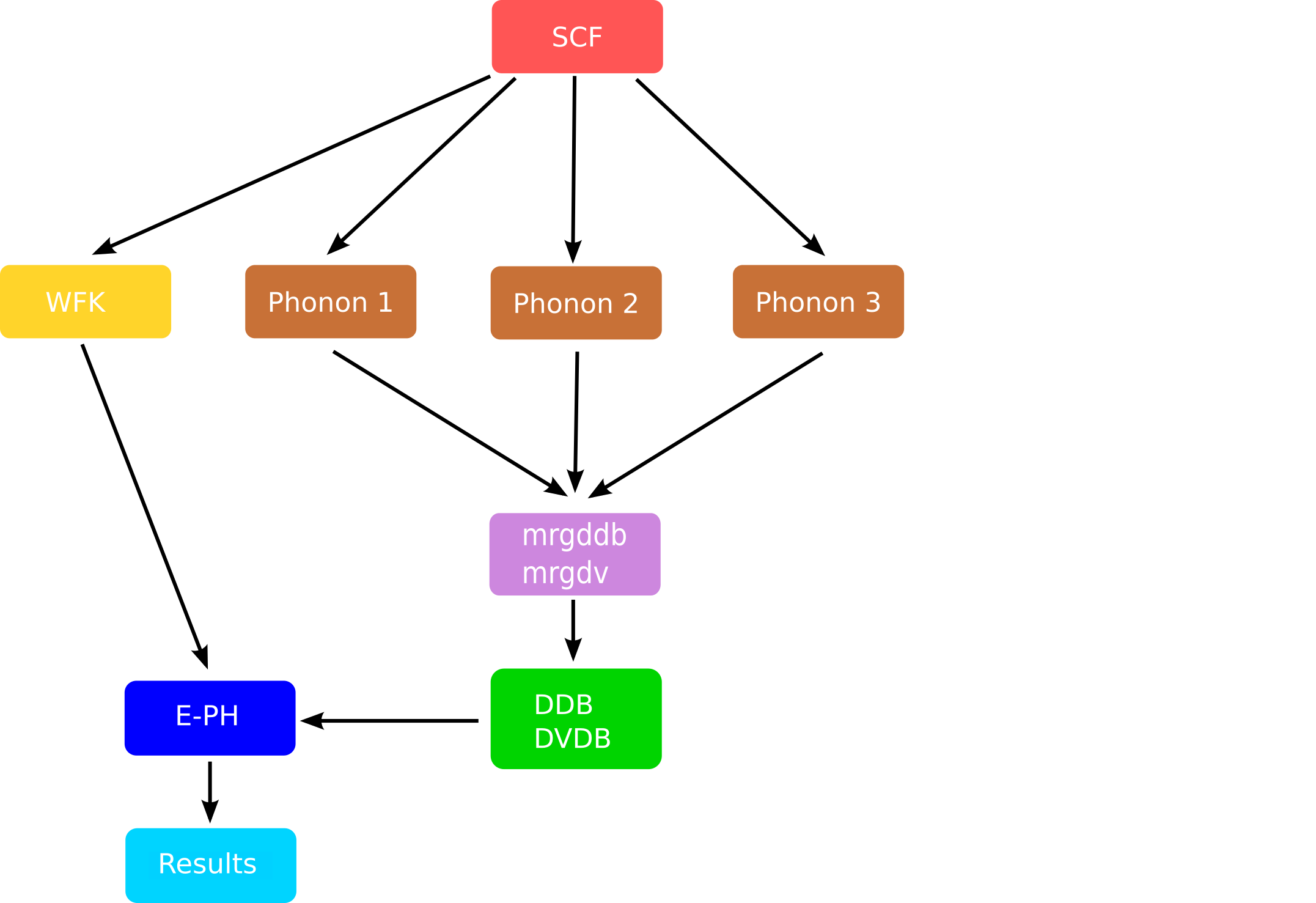
The mrgddb and mrgdv are Fortran executables whose main goal is to merge the partial files
obtained at the end of a single DFPT run for given q-point and atomic perturbation
and produce the final database required by the EPH code.
Note that, for each quasi-momentum $\kk$, the self-energy $\Sigma_{n\kk}$ is given by an integral over the BZ. This means that:
The WFK file must contain the $\kk$-points and the bands where the QP corrections are wanted as well as enough empty state to perform the summation over bands.
The code can (Fourier) interpolate the phonon frequencies and the DFPT potentials over an arbitrarily dense q-mesh. Still, for fixed $k$-point, the code requires the ab-initio KS states at $\kk$ and $\kpq$. Providing a WKF file on a k-mesh that fulfills this requirement is responsability of the user.
Since we are computing the contribution to the electron self-energy due to the interaction with phonons,
it is not surprising to encounter variables that are also used in the $GW$ code.
More specifically, one can use the nkptgw, kptgw, bdgw variables to select
the electronic states for which the QP corrections are wanted (see also gw_qprange)
while zcut defines for the complex shift.
If symsigma is set to 1, the code takes advantage of symmetries to reduce the BZ integral to an appropriate
irreducible wedge defined by the little group of the k-point (calculations at $\Gamma$ are therefore
much faster than for other low-symmetry k-points).
Suggested references
You might find additional material, related to the present section, in the following references:
Building a Flow for EPH self-energy calculations
Before starting, we need to import the python modules used in this notebook:
# Use this at the beginning of your script so that your code will be compatible with python3
from __future__ import print_function, division, unicode_literals

import numpy as np
import warnings
warnings.filterwarnings("ignore") # to get rid of deprecation warnings

from abipy import abilab
abilab.enable_notebook() # This line tells AbiPy we are running inside a notebook
import abipy.flowtk as flowtk

# This line configures matplotlib to show figures embedded in the notebook.
# Replace `inline` with `notebook` in classic notebook
%matplotlib inline

# Option available in jupyterlab. See https://github.com/matplotlib/jupyter-matplotlib
#%matplotlib widget
and a function from the lesson_sigeph module that will build our AbiPy flow.
from lesson_sigeph import build_flow
abilab.print_source(build_flow)
def build_flow(options):
    """
    C in diamond structure. Very rough q-point mesh, low ecut, completely unconverged.
    The flow computes the ground state density and a WFK file on a 8x8x8 k-mesh including
    empty states needed for the self-energy. Then all the independent atomic perturbations
    for the irreducible qpoints in a 4x4x4 grid are obtained with DFPT.
    Finally, we enter the EPH driver to compute the EPH self-energy.
    """
    workdir = options.workdir if (options and options.workdir) else "flow_diamond"

    # Define structure explicitly.
    structure = abilab.Structure.from_abivars(
        acell=3*[6.70346805],
        rprim=[0.0, 0.5, 0.5,
               0.5, 0.0, 0.5,
               0.5, 0.5, 0.0],
        typat=[1, 1],
        xred=[0.0, 0.0, 0.0, 0.25, 0.25, 0.25],
        ntypat=1,
        znucl=6,
    )

    # Initialize input from structure and norm-conserving pseudo provided by AbiPy.
    gs_inp = abilab.AbinitInput(structure, pseudos="6c.pspnc")

    # Set basic variables for GS part.
    gs_inp.set_vars(
        ecut=25.0,          # Too low, shout be ~30
        nband=4,
        tolvrs=1e-8,
    )

    # The kpoint grid is minimalistic to keep the calculation manageable.
    # The q-mesh for phonons must be a submesh of this one.
    gs_inp.set_kmesh(
        ngkpt=[8, 8, 8],
        shiftk=[0.0, 0.0, 0.0],
    )

    # Build new input for NSCF calculation with k-path (automatically selected by AbiPy)
    # Used to plot the KS band structure and interpolate the QP corrections.
    nscf_kpath_inp = gs_inp.new_with_vars(
        nband=8,
        tolwfr=1e-16,
        iscf=-2,
    )
    nscf_kpath_inp.set_kpath(ndivsm=10)

    # Build another NSCF input with k-mesh and empty states.
    # This step generates the WFK file used to build the EPH self-energy.
    nscf_empty_kmesh_inp = gs_inp.new_with_vars(
        nband=210,     # Too low. ~300
        nbdbuf=10,     # Reduces considerably the time needed to converge empty states!
        tolwfr=1e-16,
        iscf=-2,
    )

    # Create empty flow.
    flow = flowtk.Flow(workdir=workdir)

    # Register GS + band structure parts in the first work
    work0 = flowtk.BandStructureWork(gs_inp, nscf_kpath_inp, dos_inputs=[nscf_empty_kmesh_inp])
    flow.register_work(work0)

    # Generate Phonon work with 4x4x4 q-mesh
    # Reuse variables from GS input and let AbiPy handle the generation of the input files
    # Note that the q-point grid is a sub-grid of the k-point grid (here 8x8x8)
    ddb_ngqpt = [4, 4, 4]
    ph_work = flowtk.PhononWork.from_scf_task(work0[0], ddb_ngqpt, is_ngqpt=True,
                                              tolerance={"tolvrs": 1e-6})  # This to speedup DFPT
    flow.register_work(ph_work)

    # Build template for self-energy calculation. See also v8/Input/t44.in
    # The k-points must be in the WFK file
    #
    eph_inp = gs_inp.new_with_vars(
        optdriver=7,             # Enter EPH driver.
        eph_task=4,              # Activate computation of EPH self-energy.
        ddb_ngqpt=ddb_ngqpt,     # q-mesh used to produce the DDB file (must be consistent with DDB data)
        nkptgw=1,
        kptgw=[0, 0, 0],
        bdgw=[1, 8],
        # For more k-points...
        #nkptgw=2,
        #kptgw=[0, 0, 0, 0.5, 0, 0],
        #bdgw=[1, 8, 1, 8],
        tmesh=[0, 200, 5],    # (start, step, num)
        zcut="0.2 eV",        # Too large. needed to get reasonable results due to coarse q-mesh.
        nfreqsp=301,          # Compute A(w)
    )

    # Set q-path for Fourier interpolation of phonons.
    eph_inp.set_qpath(10)

    # Set q-mesh for phonons DOS.
    eph_inp.set_phdos_qmesh(nqsmall=16, method="tetra")

    # EPH part requires the GS WFK, the DDB file with all perturbations
    # and the database of DFPT potentials (already merged by PhononWork)
    deps = {work0[2]: "WFK", ph_work: ["DDB", "DVDB"]}

    # Now we use the EPH template to perform a convergence study in which
    # we change the q-mesh used to integrate the self-energy and the number of bands.
    # The code will activate the Fourier interpolation of the DFPT potentials if eph_ngqpt_fine != ddb_ngqpt

    for eph_ngqpt_fine in [[4, 4, 4], [8, 8, 8]]:
        # Create empty work to contain EPH tasks with this value of eph_ngqpt_fine
        eph_work = flow.register_work(flowtk.Work())
        for nband in [100, 150, 200]:
            new_inp = eph_inp.new_with_vars(eph_ngqpt_fine=eph_ngqpt_fine, nband=nband)
            eph_work.register_eph_task(new_inp, deps=deps)

    flow.allocate()

    return flow
OK, the function is a little bit long but it is normal as we are computing in a single workflow the electronic properties, the vibrational spectrum and the electron-phonon self-energy by varying the number of q-points and the number of empty states.
Note that we have already encountered similar flows in the previous AbiPy lessons.
The calculation of electronic band structures is
discussed in
lesson_base3,
an example of Flow for phonon calculations is given in
lesson_dfpt.
An AbiPy Flow for the computation of $G_0W_0$ corrections is discussed in
lesson_g0w0.
The novelty is represented by the generation of the EphTasks
in which we have to specify several variables related to phonons and the e-ph self-energy.
For your convenience, we have grouped the variables used in the EphTask in sub-groups:

Hopefully things will become clearer if we build the flow and start to play with it:
flow = build_flow(options=None)
flow.show_info()
<Flow, node_id=242715, workdir=flow_diamond>
Number of works: 4, total number of tasks: 23
Number of tasks with a given class:

Task Class      Number
------------  --------
ScfTask              1
NscfTask             2
PhononTask          14
EphTask              6
We now print the input of the last EphTask.
Please read carefully the documentation of the variables, in particular
those in the vargw, varrf and vareph sections.
print(flow[-1][-1])
flow[-1][-1].input
<EphTask, node_id=242751, workdir=flow_diamond/w3/t2>
#### SECTION: basic
##############################################
ecut 25.0
nband 200
tolvrs 1e-08
ngkpt 8 8 8
kptopt 1
nshiftk 1
shiftk 0.0 0.0 0.0
##############################################
#### SECTION: eph
##############################################
eph_task 4
ddb_ngqpt 4 4 4
tmesh 0 200 5
ph_ndivsm 10
ph_nqpath 12
ph_qpath
0.0 0.0 0.0
0.5 0.0 0.5
0.5 0.25 0.75
0.375 0.375 0.75
0.0 0.0 0.0
0.5 0.5 0.5
0.625 0.25 0.625
0.5 0.25 0.75
0.5 0.5 0.5
0.375 0.375 0.75
0.625 0.25 0.625
0.5 0.0 0.5
ph_intmeth 2
ph_wstep 0.0001 eV
ph_ngqpt 16 16 16
ph_qshift 0 0 0
ph_nqshift 1
eph_ngqpt_fine 8 8 8
##############################################
#### SECTION: gstate
##############################################
optdriver 7
##############################################
#### SECTION: gw
##############################################
nkptgw 1
kptgw 0.0000000000 0.0000000000 0.0000000000
bdgw 1 8
zcut 0.2 eV
nomegasf 301
##############################################
#### STRUCTURE
##############################################
natom 2
ntypat 1
typat 1 1
znucl 6
xred
0.0000000000 0.0000000000 0.0000000000
0.2500000000 0.2500000000 0.2500000000
acell 1.0 1.0 1.0
rprim
0.0000000000 3.3517340250 3.3517340250
3.3517340250 0.0000000000 3.3517340250
3.3517340250 3.3517340250 0.0000000000
As usual, it is much easier to understand what is happening if we plot a graph
with the individual tasks and their connections.
Since there are several nodes in our graph, we first focus on the EPH part
and then we "zoom-out" to unveil the entire workflow.
Let's have a look at the parents of the last EphTask with:
flow[-1][-1].get_graphviz()
The graph shows that the EphTask uses the WFK produced by a NSCF calculation
as well as two other files generated by the PhononWork.
If this is not the first time you run DFPT calculations with Abinit, you already know that the DDB
is essentially a text file with the independent entries of the dynamical matrix.
This file is usually produced by merging partial DDB files with the mrgddb utility.
For further information about the DDB see this notebook.
The DVDB, on the other hand, is a Fortran binary file containing an independent set
of DFPT potentials (actually the first-order variation of the self-consistent KS potential
due to an atomic perturbation characterized by a q-point and the [idir, ipert] pair).
The DVDB is generated by merging the POT files produced at the end of the DFPT run
with the mrgdv tool.
Now let's turn our attention to the last Work:
flow[-1].get_graphviz()
As you can see, this section of the flow consists of three EphTasks, all with the same parents.
This is the part that computes the e-ph self-energy with a fixed q-mesh and different values of nband.
We can easily check this with:
print("nband:", [task.input["nband"] for task in flow[-1]])
print("q-mesh for self-energy:", [task.input["eph_ngqpt_fine"] for task in flow[-1]])
nband: [100, 150, 200]
q-mesh for self-energy: [[8, 8, 8], [8, 8, 8], [8, 8, 8]]
or, alternatvely, we select the last work and call get_vars_dataframe with the list of variable names:
flow[-1].get_vars_dataframe("nband", "eph_ngqpt_fine")
| nband | eph_ngqpt_fine | class | |
|---|---|---|---|
| w3_t0 | 100 | [8, 8, 8] | EphTask |
| w3_t1 | 150 | [8, 8, 8] | EphTask |
| w3_t2 | 200 | [8, 8, 8] | EphTask |
There is another work made of EphTasks with similar organization, the only difference being
that we use the ab-initio q-mesh for the DFPT potentials (no Fourier interpolation here).
print("nband:", [task.input["nband"] for task in flow[-2]])
print("q-mesh for self-energy:", [task.input["eph_ngqpt_fine"] for task in flow[-2]])
nband: [100, 150, 200]
q-mesh for self-energy: [[4, 4, 4], [4, 4, 4], [4, 4, 4]]
flow[-2].get_vars_dataframe("nband", "eph_ngqpt_fine")
| nband | eph_ngqpt_fine | class | |
|---|---|---|---|
| w2_t0 | 100 | [4, 4, 4] | EphTask |
| w2_t1 | 150 | [4, 4, 4] | EphTask |
| w2_t2 | 200 | [4, 4, 4] | EphTask |
At this point, we should have a good understanding of the input files required by the EphTasks.
There is only one point missing! How do we get the WFK, DDB, DVDB files?
Well, in the old days we used to write several input files one for each q-point in the IBZ, link files and merge the intermediate results manually but now we can use python to automate the entire procedure:
flow.get_graphviz()
More specifically, the q-mesh associated to the
DDB (DVDB) must be a submesh of the k-mesh for electrons.
Moreover the EPH code can compute self-energy corrections only for the states that are available in the WFK file.
Now we can generate the directories and the input files of the Flow by executing the
lesson_sigeph.py script that will generate the flow_diamond directory with all the input
files required by the calculation.
Then use the abirun.py script to launch the calculation with the scheduler:
abirun.py flow_diamond scheduler
You may want to run this example in the terminal if you have already installed and configured AbiPy and Abinit on your machine. The calculation requires ~8 minutes on a poor 1.7 GHz Intel Core i5 (2 minutes for all the EPH tasks, the rest for the DFPT section).
If you prefer to skip this part, jump to next section in which we focus on the post-processing of the results. Note that the output files are already available in the github repository so it is possible to play with the AbiPy post-processing tools without having to run the flow. In particular, one can use the command line and the commands:
abiopen.py FILE
to open the file inside ipython,
abiopen.py out_SIGEPH.nc --expose
to visualize the self-energy results and finally,
abicomp.py sigeph flow_diamond/w3/
to compare multiple SIGEPH.nc files with the robot inside ipython.
!find flow_diamond/ -name "out_GSR.nc"
flow_diamond//w0/t2/outdata/out_GSR.nc
flow_diamond//w0/t1/outdata/out_GSR.nc
flow_diamond//w0/t0/outdata/out_GSR.nc
The task w0/t0 computed the electronic band structure on a high-symmetry k-path.
Let's plot the bands with:
with abilab.abiopen("flow_diamond/w0/t1/outdata/out_GSR.nc") as gsr:
    ebands_kpath = gsr.ebands

ebands_kpath.plot(with_gaps=True);

It's not surprising to see that diamond is a indirect gap semiconductor.
The KS band structure gives a direct gap at $\Gamma$ of ~5.6 eV while the fundamental gap
is ~4.2 eV (VBM at $\Gamma$, CBM at ~[+0.357, +0.000, +0.357] in reduced coordinates).
These values have been computer by ApiPy on the basis of the k-path employed to compute the band structure
in the NscfTask:
print(ebands_kpath)
================================= Structure =================================
Full Formula (C2)
Reduced Formula: C
abc   :   2.508336   2.508336   2.508336
angles:  60.000000  60.000000  60.000000
Sites (2)
  #  SP       a     b     c  cartesian_forces
---  ----  ----  ----  ----  -----------------------------------------------------------
  0  C     0     0     0     [5.14220675e+101 5.14220675e+101 5.14220675e+101] eV ang^-1
  1  C     0.25  0.25  0.25  [5.14220675e+101 5.14220675e+101 5.14220675e+101] eV ang^-1

Abinit Spacegroup: spgid: 227, num_spatial_symmetries: 48, has_timerev: True, symmorphic: True

Number of electrons: 8.0, Fermi level: 12.743 (eV)
nsppol: 1, nkpt: 198, mband: 8, nspinor: 1, nspden: 1
smearing scheme: none (occopt 1), tsmear_eV: 0.272
Direct gap:
    Energy: 5.617 (eV)
    Initial state: spin: 0, kpt: [+0.000, +0.000, +0.000], name: $\Gamma$, weight: 0.000, band: 3, eig: 12.743, occ: 2.000
    Final state:   spin: 0, kpt: [+0.000, +0.000, +0.000], name: $\Gamma$, weight: 0.000, band: 4, eig: 18.361, occ: 0.000
Fundamental gap:
    Energy: 4.205 (eV)
    Initial state: spin: 0, kpt: [+0.000, +0.000, +0.000], name: $\Gamma$, weight: 0.000, band: 3, eig: 12.743, occ: 2.000
    Final state:   spin: 0, kpt: [+0.357, +0.000, +0.357], weight: 0.000, band: 4, eig: 16.949, occ: 0.000
Bandwidth: 21.540 (eV)
Valence maximum located at:
    spin: 0, kpt: [+0.000, +0.000, +0.000], name: $\Gamma$, weight: 0.000, band: 3, eig: 12.743, occ: 2.000
Conduction minimum located at:
    spin: 0, kpt: [+0.357, +0.000, +0.357], weight: 0.000, band: 4, eig: 16.949, occ: 0.000

TIP: Call set_fermie_to_vbm() to set the Fermi level to the VBM if this is a non-magnetic semiconductor
In the NscfTask w0/t2 we have computed the KS eigenstates including several empty states.
This is the WFK file we are going to use to build the EPH self-energy.
Let's plot the bands in the IBZ and the associated DOS with:
with abilab.abiopen("flow_diamond/w0/t2/outdata/out_GSR.nc") as gsr:
    ebands_4sigma = gsr.ebands

# 8x8x8 is too coarse to get nice DOS so we increase the gaussian smearing
# (we are mainly interested in the possible presence of ghost states --> sharp peaks)
ebands_4sigma.plot_with_edos(ebands_4sigma.get_edos(width=0.6));

The figure shows that our value of nband correspond to ~400 eV above the valence band maximum (VBM).
Note that it is always a good idea to look at the behaviour of the high-energy states when running self-energy calculations, especially the first time you use a new pseudopotential.
Ghost states, indeed, can appear somewhere in the high-energy region causing sharp peaks in the DOS. The presence of these high-energy ghosts is not clearly seen in standard GS calculations but they can have drammatic consequences for many-body calculations based on sum-over-states approaches.
This is one of the reasons why the pseudopotentials of the pseudo-dojo project have been explicitly tested for the presence of ghost states in the empty region (see here for further details)
Vibrational properties
Now we turn our attention to the vibrational properties.
AbiPy has already merged all the independent atomic perturbations in flow_diamond/w1/outdata/out_DDB:
!find flow_diamond/ -name "out_DDB"
flow_diamond//w0/t0/outdata/out_DDB
flow_diamond//w1/t11/outdata/out_DDB
flow_diamond//w1/t10/outdata/out_DDB
flow_diamond//w1/t5/outdata/out_DDB
flow_diamond//w1/t2/outdata/out_DDB
flow_diamond//w1/t3/outdata/out_DDB
flow_diamond//w1/t4/outdata/out_DDB
flow_diamond//w1/t12/outdata/out_DDB
flow_diamond//w1/t13/outdata/out_DDB
flow_diamond//w1/outdata/out_DDB
flow_diamond//w1/t1/outdata/out_DDB
flow_diamond//w1/t6/outdata/out_DDB
flow_diamond//w1/t8/outdata/out_DDB
flow_diamond//w1/t9/outdata/out_DDB
flow_diamond//w1/t7/outdata/out_DDB
flow_diamond//w1/t0/outdata/out_DDB
This is the input file for mrgddb produced automatically by python:
!cat flow_diamond//w1/outdata/mrgddb.stdin
/Users/gmatteo/git_repos/abitutorials/abitutorials/sigeph/flow_diamond/w1/outdata/out_DDB
DDB file merged by PhononWork on Wed Sep 30 03:53:31 2020
14
/Users/gmatteo/git_repos/abitutorials/abitutorials/sigeph/flow_diamond/w1/t0/outdata/out_DDB
/Users/gmatteo/git_repos/abitutorials/abitutorials/sigeph/flow_diamond/w1/t1/outdata/out_DDB
/Users/gmatteo/git_repos/abitutorials/abitutorials/sigeph/flow_diamond/w1/t2/outdata/out_DDB
/Users/gmatteo/git_repos/abitutorials/abitutorials/sigeph/flow_diamond/w1/t3/outdata/out_DDB
/Users/gmatteo/git_repos/abitutorials/abitutorials/sigeph/flow_diamond/w1/t4/outdata/out_DDB
/Users/gmatteo/git_repos/abitutorials/abitutorials/sigeph/flow_diamond/w1/t5/outdata/out_DDB
/Users/gmatteo/git_repos/abitutorials/abitutorials/sigeph/flow_diamond/w1/t6/outdata/out_DDB
/Users/gmatteo/git_repos/abitutorials/abitutorials/sigeph/flow_diamond/w1/t7/outdata/out_DDB
/Users/gmatteo/git_repos/abitutorials/abitutorials/sigeph/flow_diamond/w1/t8/outdata/out_DDB
/Users/gmatteo/git_repos/abitutorials/abitutorials/sigeph/flow_diamond/w1/t9/outdata/out_DDB
/Users/gmatteo/git_repos/abitutorials/abitutorials/sigeph/flow_diamond/w1/t10/outdata/out_DDB
/Users/gmatteo/git_repos/abitutorials/abitutorials/sigeph/flow_diamond/w1/t11/outdata/out_DDB
/Users/gmatteo/git_repos/abitutorials/abitutorials/sigeph/flow_diamond/w1/t12/outdata/out_DDB
/Users/gmatteo/git_repos/abitutorials/abitutorials/sigeph/flow_diamond/w1/t13/outdata/out_DDB
The first line gives the name of the output DDB file followed by a title, the number of partial DDB files we want to merge and their path.
A similar input file must be provided to mrgdv, the only difference is that DDB files are not replaced
by POT* files with the SCF part of the DFPT potential (Warning: Unlike the out_DDB files,
the out_DVDB file and the associated mrgdvdb.stdin files are available
in the present tutorial only if you have actually issued abirun.py flow_diamond scheduler above.
Still, the files needed beyond the two next commands are available by default, so that you can continue to examine this tutorial.)
!find flow_diamond/ -name "out_DVDB"
flow_diamond//w1/outdata/out_DVDB
!cat flow_diamond//w1/outdata/mrgdvdb.stdin
/Users/gmatteo/git_repos/abitutorials/abitutorials/sigeph/flow_diamond/w1/outdata/out_DVDB
14
/Users/gmatteo/git_repos/abitutorials/abitutorials/sigeph/flow_diamond/w1/t0/outdata/out_POT1
/Users/gmatteo/git_repos/abitutorials/abitutorials/sigeph/flow_diamond/w1/t1/outdata/out_POT1
/Users/gmatteo/git_repos/abitutorials/abitutorials/sigeph/flow_diamond/w1/t2/outdata/out_POT2
/Users/gmatteo/git_repos/abitutorials/abitutorials/sigeph/flow_diamond/w1/t3/outdata/out_POT1
/Users/gmatteo/git_repos/abitutorials/abitutorials/sigeph/flow_diamond/w1/t4/outdata/out_POT2
/Users/gmatteo/git_repos/abitutorials/abitutorials/sigeph/flow_diamond/w1/t5/outdata/out_POT1
/Users/gmatteo/git_repos/abitutorials/abitutorials/sigeph/flow_diamond/w1/t6/outdata/out_POT1
/Users/gmatteo/git_repos/abitutorials/abitutorials/sigeph/flow_diamond/w1/t7/outdata/out_POT2
/Users/gmatteo/git_repos/abitutorials/abitutorials/sigeph/flow_diamond/w1/t8/outdata/out_POT3
/Users/gmatteo/git_repos/abitutorials/abitutorials/sigeph/flow_diamond/w1/t9/outdata/out_POT1
/Users/gmatteo/git_repos/abitutorials/abitutorials/sigeph/flow_diamond/w1/t10/outdata/out_POT3
/Users/gmatteo/git_repos/abitutorials/abitutorials/sigeph/flow_diamond/w1/t11/outdata/out_POT1
/Users/gmatteo/git_repos/abitutorials/abitutorials/sigeph/flow_diamond/w1/t12/outdata/out_POT1
/Users/gmatteo/git_repos/abitutorials/abitutorials/sigeph/flow_diamond/w1/t13/outdata/out_POT2
Let's open the DDB file with:
ddb = abilab.abiopen("flow_diamond/w1/outdata/out_DDB")
print(ddb)
================================= File Info =================================
Name: out_DDB
Directory: /Users/gmatteo/git_repos/abitutorials/abitutorials/sigeph/flow_diamond/w1/outdata
Size: 55.08 kb
Access Time: Wed Sep 30 04:00:47 2020
Modification Time: Wed Sep 30 03:53:31 2020
Change Time: Wed Sep 30 03:53:31 2020

================================= Structure =================================
Full Formula (C2)
Reduced Formula: C
abc   :   2.508336   2.508336   2.508336
angles:  60.000000  60.000000  60.000000
Sites (2)
  #  SP       a     b     c
---  ----  ----  ----  ----
  0  C     0     0     0
  1  C     0.25  0.25  0.25

Abinit Spacegroup: spgid: 0, num_spatial_symmetries: 48, has_timerev: True, symmorphic: True

================================== DDB Info ==================================

Number of q-points in DDB: 8
guessed_ngqpt: [4 4 4] (guess for the q-mesh divisions made by AbiPy)
ecut = 25.000000, ecutsm = 0.000000, nkpt = 260, nsym = 48, usepaw = 0
nsppol 1, nspinor 1, nspden 1, ixc = 1, occopt = 1, tsmear = 0.010000

Has total energy: False, Has forces: False
Has stress tensor: False

Has (at least one) atomic pertubation: True
Has (at least one diagonal) electric-field perturbation: False
Has (at least one) Born effective charge: False
Has (all) strain terms: False
Has (all) internal strain terms: False
Has (all) piezoelectric terms: False
and then invoke anaddb to compute phonon bands and DOS:
phbst, phdos = ddb.anaget_phbst_and_phdos_files()
Finally we plot the results with:
phbst.phbands.plot_with_phdos(phdos);

The maximum phonon frequency is ~0.17 eV that is much smaller that the KS fundamental gap. This means that at T=0 we cannot have scattering processes between two electronic states in which only one phonon is involved. This however does not mean that the electronic properties will not be renormalized by the EPH interaction, even at T=0 (zero-point motion effect).
So far, we managed to generate a WFK with empty states on a 8x8x8 k-mesh,
and a pair of DDB-DVDB files on a 4x4x4 q-mesh.
We can now finally turn our attention to the EPH self-energy.
E-PH self-energy
Let's focus on the output files produced by the first EphTask in w2/t0:
!ls flow_diamond/w2/t0/outdata
out_EBANDS.agr  out_PHBANDS.agr out_PHDOS.nc
out_OUT.nc      out_PHBST.nc    out_SIGEPH.nc
where:
- out_PHBST.nc: phonon band structure along the q-path
- out_PHDOS.nc: phonon DOS and projections over atoms and directions
- out_SIGEPH.nc: $\Sigma^{eph}_{nk\sigma}(T)$ matrix elements for different temperatures $T$
There are several physical properties stored in the SIGEPH file.
As usual, we can use abiopen to open the file and print(abifile) to get a quick summary
of the most important results.
Let's open the file obtained with the 8x8x8 q-mesh and 200 bands (our best calculation):
#sigeph = abilab.abiopen("flow_diamond/w2/t0/outdata/out_SIGEPH.nc")
sigeph = abilab.abiopen("flow_diamond/w3/t2/outdata/out_SIGEPH.nc")
print(sigeph)
================================= File Info =================================
Name: out_SIGEPH.nc
Directory: /Users/gmatteo/git_repos/abitutorials/abitutorials/sigeph/flow_diamond/w3/t2/outdata
Size: 498.37 kb
Access Time: Wed Sep 30 04:00:53 2020
Modification Time: Wed Sep 30 03:53:56 2020
Change Time: Wed Sep 30 03:53:56 2020

================================= Structure =================================
Full Formula (C2)
Reduced Formula: C
abc   :   2.508336   2.508336   2.508336
angles:  60.000000  60.000000  60.000000
Sites (2)
  #  SP       a     b     c
---  ----  ----  ----  ----
  0  C     0     0     0
  1  C     0.25  0.25  0.25

Abinit Spacegroup: spgid: 0, num_spatial_symmetries: 48, has_timerev: True, symmorphic: True

============================= KS Electron Bands =============================
Number of electrons: 8.0, Fermi level: 12.743 (eV)
nsppol: 1, nkpt: 29, mband: 210, nspinor: 1, nspden: 1
smearing scheme: none (occopt 1), tsmear_eV: 0.272
Direct gap:
    Energy: 5.617 (eV)
    Initial state: spin: 0, kpt: [+0.000, +0.000, +0.000], weight: 0.002, band: 3, eig: 12.743, occ: 2.000
    Final state:   spin: 0, kpt: [+0.000, +0.000, +0.000], weight: 0.002, band: 4, eig: 18.361, occ: 0.000
Fundamental gap:
    Energy: 4.209 (eV)
    Initial state: spin: 0, kpt: [+0.000, +0.000, +0.000], weight: 0.002, band: 3, eig: 12.743, occ: 2.000
    Final state:   spin: 0, kpt: [+0.375, +0.375, +0.000], weight: 0.012, band: 4, eig: 16.952, occ: 0.000
Bandwidth: 21.540 (eV)
Valence maximum located at:
    spin: 0, kpt: [+0.000, +0.000, +0.000], weight: 0.002, band: 3, eig: 12.743, occ: 2.000
Conduction minimum located at:
    spin: 0, kpt: [+0.375, +0.375, +0.000], weight: 0.012, band: 4, eig: 16.952, occ: 0.000

TIP: Call set_fermie_to_vbm() to set the Fermi level to the VBM if this is a non-magnetic semiconductor


============================ SigmaEPh calculation ============================
Calculation type: Real + Imaginary part of SigmaEPh
Number of k-points in Sigma_{nk}: 1
sigma_ngkpt: [0 0 0], sigma_erange: [0. 0.]
Max bstart: 0, min bstop: 8
Initial ab-initio q-mesh:
	ngqpt: [8 8 8], with nqibz: 29
q-mesh for self-energy integration (eph_ngqpt_fine): [8 8 8]
k-mesh for electrons:
	mpdivs: [8 8 8] with shifts [[0. 0. 0.]] and kptopt: 1
Number of bands included in e-ph self-energy sum: 200
zcut: 0.00735 (Ha), 0.200 (eV)
Number of temperatures: 5, from 0.0 to 800.0 (K)
symsigma: 1
Has Eliashberg function: False
Has Spectral function: True

Printing QP results for 2 temperatures. Use --verbose to print all results.

KS, QP (Z factor) and on-the-mass-shell (OTMS) direct gaps in eV for T = 0.0 K:
  Spin  k-point                              KS_gap    QPZ_gap    QPZ - KS    OTMS_gap    OTMS - KS
------  ---------------------------------  --------  ---------  ----------  ----------  -----------
     0  [+0.000, +0.000, +0.000] $\Gamma$     5.617      5.322      -0.295       5.264       -0.353


KS, QP (Z factor) and on-the-mass-shell (OTMS) direct gaps in eV for T = 800.0 K:
  Spin  k-point                              KS_gap    QPZ_gap    QPZ - KS    OTMS_gap    OTMS - KS
------  ---------------------------------  --------  ---------  ----------  ----------  -----------
     0  [+0.000, +0.000, +0.000] $\Gamma$     5.617      5.243      -0.374       5.146       -0.471
The output reveals that the direct QP gaps are smaller than the corresponding KS values, even at $T=0$. Still it is difficult to understand what is happening without a graphical representation of the results. Let's use matplotlib to plot the difference between the QP and the KS direct gap at $\Gamma$ as a function or T:
sigeph.plot_qpgaps_t();

In diamond, the EPH interaction at T=0 decreases the direct gap at $\Gamma$ with respect to the KS value. Moreover the QP gap decreases with T. This behaviour, however, cannot be generalized in the sense that there are systems in which the direct gap increases with T.
So far we have been focusing on the QP direct gaps but we can also look at the QP results for the CBM and the VBM:
# Valence band max
sigeph.plot_qpdata_t(spin=0, kpoint=0, band_list=[3]);

# Conduction band min
sigeph.plot_qpdata_t(spin=0, kpoint=0, band_list=[4]);

Note how the real part of the self-energy at the VBM goes up with T while the CBM goes down with T, thus explaining the behavior of the QP gap vs T observed previously (well one should also include $Z$ but the real part gives the most important contribution...)
We do not discuss the results for the imaginary part because these values requires a very dense sampling of the BZ to give reasonable results.
We can also plot the real and the imaginary part of $\Sigma_{nk}^{eph}(\omega)$ and the spectral function $A_{nk}(\omega)$ obtained for the different temperatures with:
sigma = sigeph.get_sigeph_skb(spin=0, kpoint=[0, 0, 0], band=3)
sigma.plot_tdep(xlims=[-1, 2]);

sigeph.get_sigeph_skb(spin=0, kpoint=[0, 0, 0], band=4).plot_tdep(xlims=(-1, 2));

Converging these quantities is not an easy task since they are very sensitive to the q-point sampling. Still, we can see that the spectral function has a dominant peak that is shifted with respect to the initial KS energy. The spectral function of the CBM has more structures than the VBM...
In some cases, we need to access the raw data.
For example we may want to build a table with the QP results for all bands at fixed k-point, spin.
The code below creates a pandas DataFrame and selects only the entries at 0 K.
df = sigeph.get_dataframe_sk(spin=0, kpoint=[0, 0, 0], ignore_imag=True)
df[df["tmesh"] == 0.0]
| band | e0 | re_qpe | qpeme0 | re_sig0 | imag_sig0 | ze0 | re_fan0 | dw | tmesh | |
|---|---|---|---|---|---|---|---|---|---|---|
| 0 | 0 | -8.796107 | -8.857742 | -0.061635 | -0.062745 | 0.0 | 0.982315 | -0.121061 | 0.058316 | 0.0 |
| 0 | 1 | 12.743474 | 12.866324 | 0.122850 | 0.131324 | 0.0 | 0.935473 | -0.936921 | 1.068245 | 0.0 |
| 0 | 2 | 12.743474 | 12.866324 | 0.122850 | 0.131324 | 0.0 | 0.935473 | -0.936921 | 1.068245 | 0.0 |
| 0 | 3 | 12.743474 | 12.866324 | 0.122850 | 0.131324 | 0.0 | 0.935473 | -0.936921 | 1.068245 | 0.0 |
| 0 | 4 | 18.360583 | 18.188235 | -0.172348 | -0.222156 | 0.0 | 0.775797 | -1.166413 | 0.944257 | 0.0 |
| 0 | 5 | 18.360583 | 18.188235 | -0.172348 | -0.222156 | 0.0 | 0.775797 | -1.166413 | 0.944257 | 0.0 |
| 0 | 6 | 18.360583 | 18.188235 | -0.172348 | -0.222156 | 0.0 | 0.775797 | -1.166413 | 0.944257 | 0.0 |
| 0 | 7 | 26.672500 | 26.675328 | 0.002828 | 0.004461 | 0.0 | 0.633845 | -0.080522 | 0.084983 | 0.0 |
# To plot the QP results as a function of the KS energy:
#sigeph.plot_qps_vs_e0();
# To plot KS bands and QP results:
#sigeph.plot_qpbands_ibzt();
Using SigEphRobot for convergence studies
Our initial goal was to analyze the convergence of the QP corrections as a function of nbsum.
This means that we should now collect multiple SIGEPH.nc files, extract the data,
order the results and visualize them.
Fortunately, we can use the SigEphRobot (or the abicomp.py script)
to automate the most boring and repetitive operations.
The code below, for instance, tells our robot to open all the SIGEPH files
located within flow_diamond/w2 (fixed q-mesh, different nband).
The syntax used to specify multiple directories should be familiar to Linux users:
robot_bsum = abilab.SigEPhRobot.from_dir_glob("flow_diamond/w2/t*/outdata/")
robot_bsum
- flow_diamond/w2/t2/outdata/out_SIGEPH.nc
- flow_diamond/w2/t1/outdata/out_SIGEPH.nc
- flow_diamond/w2/t0/outdata/out_SIGEPH.nc
Let's change the labels of the files by replacing file paths with strings constructed
from nbsum:
robot_bsum.remap_labels(lambda sigeph: "nbsum: %d" % sigeph.nbsum)
OrderedDict([('nbsum: 200', 'flow_diamond/w2/t2/outdata/out_SIGEPH.nc'),
             ('nbsum: 150', 'flow_diamond/w2/t1/outdata/out_SIGEPH.nc'),
             ('nbsum: 100', 'flow_diamond/w2/t0/outdata/out_SIGEPH.nc')])
and check that everything is OK by printing the convergence parameters:
robot_bsum.get_params_dataframe()
| nbsum | zcut | symsigma | nqbz | nqibz | ddb_nqbz | eph_nqbz_fine | ph_nqbz | eph_intmeth | eph_fsewin | eph_fsmear | eph_extrael | eph_fermie | |
|---|---|---|---|---|---|---|---|---|---|---|---|---|---|
| nbsum: 200 | 200 | 0.007349865079592465 | 1 | 64 | 8 | 64 | 64 | 4096 | 1 | 0.04 | 0.01 | 0.0 | 0.0 |
| nbsum: 150 | 150 | 0.007349865079592465 | 1 | 64 | 8 | 64 | 64 | 4096 | 1 | 0.04 | 0.01 | 0.0 | 0.0 |
| nbsum: 100 | 100 | 0.007349865079592465 | 1 | 64 | 8 | 64 | 64 | 4096 | 1 | 0.04 | 0.01 | 0.0 | 0.0 |
As expected, the only parameter that is changing in this set of netcdf files is nbsum.
Now all the files are in memory and we can start our convergence study.
To plot the convergence of QP gaps vs the nbsum parameter, use:
robot_bsum.plot_qpgaps_convergence(sortby="nbsum", itemp=0);

The convergence of the QP gaps versus nbsum is not variational
and very slow: the same run with 20 bands (not shown here) would give completely different results.
Note that QP gaps (energy differences) are usually easier to converge than absolute QP energies.
A similar behaviour is observed in $GW$ calculations as well.
We can also analyze the convergence of the individual QP terms for given $(\sigma, {\bf{k}}, n)$ with:
robot_bsum.plot_qpdata_conv_skb(spin=0, kpoint=(0, 0, 0), band=3, sortby="nbsum");

#robot_bsum.plot_qpdata_conv_skb(spin=0, kpoint=(0, 0, 0), band=4, sortby="nbsum");
and perform a similar analysis for $\Sigma^{eph}_{n{\bf k}}(\omega)$ and $A_{n{\bf k}}(\omega)$:
robot_bsum.plot_selfenergy_conv(spin=0, kpoint=(0 , 0, 0), band=4, itemp=0);

Note how the largest variations are observed in the real part of the self-energy while the imaginary part is rather insensitive to the number of empty states. Why?
Convergence study with respect to nbsum and nqibz
In the previous section, we have analyzed the convergence of the QP results as a function of nbsum
for a fixed q-point mesh.
The main conclusion was that the convergence with respect to the number of bands is slow
and that even 200 bands are not enough to converge the QP gap.
Here we use all the SIGEPH.nc files produced by the flow to study
how the final results depend on nbsum and nqibz.
The main goal is to understand whether these two parameters are correlated or not. In other words we want to understand whether we really need to perform a convergence study in which both parameters are increased or whether we can assume some sort of weak correlation that allows us to decouple the two convergence studies.
Let's start by loading all the SIGPEH.nc files located inside flow_diamond with:
robot_qb = abilab.SigEPhRobot.from_dir("flow_diamond")
robot_qb
- w3/t2/outdata/out_SIGEPH.nc
- w3/t1/outdata/out_SIGEPH.nc
- w3/t0/outdata/out_SIGEPH.nc
- w2/t2/outdata/out_SIGEPH.nc
- w2/t1/outdata/out_SIGEPH.nc
- w2/t0/outdata/out_SIGEPH.nc
and replace the labels with:
robot_qb.remap_labels(lambda sigeph: "nbsum: %d, nqibz: %d" % (sigeph.nbsum, sigeph.nqibz))
OrderedDict([('nbsum: 200, nqibz: 29', 'w3/t2/outdata/out_SIGEPH.nc'),
             ('nbsum: 150, nqibz: 29', 'w3/t1/outdata/out_SIGEPH.nc'),
             ('nbsum: 100, nqibz: 29', 'w3/t0/outdata/out_SIGEPH.nc'),
             ('nbsum: 200, nqibz: 8', 'w2/t2/outdata/out_SIGEPH.nc'),
             ('nbsum: 150, nqibz: 8', 'w2/t1/outdata/out_SIGEPH.nc'),
             ('nbsum: 100, nqibz: 8', 'w2/t0/outdata/out_SIGEPH.nc')])
All the calculations in w2 are done with a 4x4x4 q-mesh, while in w3 we have EPH calculations
done with a 8x8x8 q-mesh.
Let's print a table with the parameters of the run, just to be sure...
robot_qb.get_params_dataframe()
| nbsum | zcut | symsigma | nqbz | nqibz | ddb_nqbz | eph_nqbz_fine | ph_nqbz | eph_intmeth | eph_fsewin | eph_fsmear | eph_extrael | eph_fermie | |
|---|---|---|---|---|---|---|---|---|---|---|---|---|---|
| nbsum: 200, nqibz: 29 | 200 | 0.007349865079592465 | 1 | 512 | 29 | 64 | 512 | 4096 | 1 | 0.04 | 0.01 | 0.0 | 0.0 |
| nbsum: 150, nqibz: 29 | 150 | 0.007349865079592465 | 1 | 512 | 29 | 64 | 512 | 4096 | 1 | 0.04 | 0.01 | 0.0 | 0.0 |
| nbsum: 100, nqibz: 29 | 100 | 0.007349865079592465 | 1 | 512 | 29 | 64 | 512 | 4096 | 1 | 0.04 | 0.01 | 0.0 | 0.0 |
| nbsum: 200, nqibz: 8 | 200 | 0.007349865079592465 | 1 | 64 | 8 | 64 | 64 | 4096 | 1 | 0.04 | 0.01 | 0.0 | 0.0 |
| nbsum: 150, nqibz: 8 | 150 | 0.007349865079592465 | 1 | 64 | 8 | 64 | 64 | 4096 | 1 | 0.04 | 0.01 | 0.0 | 0.0 |
| nbsum: 100, nqibz: 8 | 100 | 0.007349865079592465 | 1 | 64 | 8 | 64 | 64 | 4096 | 1 | 0.04 | 0.01 | 0.0 | 0.0 |
We can start to analyze the data but there is a small problem because, strictly speaking,
we are dealing with a function of two variables. (nbsum and nqibz).
Let's analyze the convergence of the QP direct gap as a function of nbsum and use the hue argument
to group results obtained with different q-meshes:
robot_qb.plot_qpgaps_convergence(sortby="nbsum", hue="nqibz", itemp=0);

The figure reveals that the largest variation is due to the q-point sampling,
nonetheless the two curves as function of nbsum have very similar trend
(they are just converging to different values)
This suggests that one could simplify considerably the convergence study by decoupling the two parameters.
In particular, one could perform an initial convergence study with respect to nbsum with a relatively coarse q-mesh
to find a reasonable value then fix nbsum and move to the convergence study with respect to the q-point sampling
and the zcut broadening.
A similar approach has been recently used by van Setten to automate $GW$ calculation.
#robot_qb.plot_qpfield_vs_e0("qpeme0", itemp=0, sortby="nbsum", hue="nqibz");
#robot_qb.plot_qpdata_conv_skb(spin=0, kpoint=(0, 0, 0), band=3, sortby="nbsum", hue="nqibz");
#robot_qb.plot_selfenergy_conv(spin=0, kpoint=(0.5, 0, 0), band=4, itemp=0, sortby="nbsum", hue="nqibz");
#robot_qb.plot_qpgaps_t(); #sortby="nbsum", plot_qpmks=True, hue="nqibz");
#robot_qb.plot_qpgaps_t(sortby="nbsum", plot_qpmks=True, hue="nqibz");
#robot_qb.plot_qpgaps_convergence(itemp=0, sortby="nbsum", hue="nqibz");
#robot_qb.plot_qpfield_vs_e0("ze0", itemp=0, sortby="nbsum", hue="nqibz");
Interpolating QP corrections with star-functions
In the previous paragraphs, we discussed how to compute the QP corrections as function of $T$ for a set of k-points in the IBZ. In many cases, however, we would like to visualize the effect of the self-energy on the electronic dispersion using a high-symmetry k-path. There are several routes to address this problem.
The most accurate method would be performing multiple self-energy calculations with different shifted k-meshes so as to sample the high-symmetry k-path and then merging the results. Alternatively, one could try to interpolate the QP energies obtained in the IBZ.
It is worth noting that the QP energies must fulfill the symmetry properties of the point group of the crystal:
\begin{equation} \epsilon({\bf k + G}) = \epsilon({\bf k}) \end{equation}and
\begin{equation} \epsilon(\mathcal O {\bf k }) = \epsilon({\bf k}) \end{equation}where $\bf{G}$ is a reciprocal lattice vector and $\mathcal{O}$ is an operation of the point group.
Therefore it is possible to employ the star-function interpolation by Shankland, Koelling and Wood in the improved version proposed by Pickett to fit the ab-initio results. This interpolation technique, by construction, passes through the initial points and satisfies the basic symmetry property of the band energies.
It should be stressed, however, that this Fourier-based method can have problems in the presence of band crossings that may cause unphysical oscillations between the ab-initio points. To reduce this spurious effect, we prefer to interpolate the QP corrections instead of the QP energies. The corrections, indeed, are usually smoother in k-space and the resulting fit is more stable.
To interpolate the QP corrections we have to provide a SIGEPH file with the QP energies computed
in the entire irreducible zone.
A netcdf file obtained with nband == 100 is already provided in the github repository.
Note that the QP corrections in this case have been obtained by setting $Z = 1$
sigeph_ibz = abilab.abiopen("ibz_SIGEPH.nc")
These are the QP energies and the KS bands in the irreducible wedge:
sigeph_ibz.plot_qpbands_ibzt();

Now we extract the KS bands along the k-path from the GSR file produced by the second NscfTask
with abilab.abiopen("flow_diamond/w0/t1/outdata/out_GSR.nc") as gsr:
    ks_ebands_kpath = gsr.ebands
Finally, we interpolate the QP corrections for the first two temperatures by calling:
tdep = sigeph_ibz.interpolate(ks_ebands_kpath=ks_ebands_kpath, itemp_list=[0, 1])
sigres.structure and ks_ebands_kpath.structures differ. Check your files!
Using: 145 star-functions. nstars/nk: 5.0
FIT vs input data: Mean Absolute Error= 2.927e-11 (meV)
Using: 145 star-functions. nstars/nk: 5.0
FIT vs input data: Mean Absolute Error= 0.000e+00 (meV)
Using: 145 star-functions. nstars/nk: 5.0
FIT vs input data: Mean Absolute Error= 3.161e-11 (meV)
Using: 145 star-functions. nstars/nk: 5.0
FIT vs input data: Mean Absolute Error= 0.000e+00 (meV)
Finally, one can plot the interpolated QP bands and the ab-initio KS dispersion with:
tdep.plot();

Let's zoom in on the region around the gap:
tdep.plot(ylims=(-1, 6));

Back to the main Index