PyTables
import addutils.toc ; addutils.toc.js(ipy_notebook=True)
PyTables is an high-performance, on-disk data container, query engine and computation kernel, with an easy-to-use interface, developed by Francesc Alted since 2002.
from addutils import css_notebook
css_notebook()
PyTables - What is it?
PyTables is a Python package wich allows dealing with HDF5 tables and:
- a binary data container for on-disk, structured data
- with support for data compression: Zlib, bzip2, LZO and Blosc
- with powerful query and indexing capabilities
- can perform out-of-core (data on-disk) operations very efficiently
- based on the standard de-facto HDF5 format
- free software (BSD license)
PyTables - What is not
- NOT a relational database replacement
- not a distributed database
- not extremely secure of safe (it's more about speed)
- not a mere HDF5 wrapper
1 The Array Object
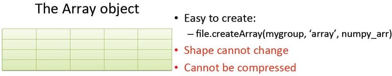
TODO: The immage above has a wrong command. The right command is file.create_array()
import numpy as np
import tables as tb
f = tb.open_file('temp/atest.h5', 'w')  # Create a new file in "write" mode
a = np.arange(50).reshape(5,10)        # Create a NumPy array
f.create_array(f.root, 'my_array1', a)     # Save the array
/my_array1 (Array(5, 10)) ''
  atom := Int64Atom(shape=(), dflt=0)
  maindim := 0
  flavor := 'numpy'
  byteorder := 'little'
  chunkshape := None
The create_array method returns a handler of the array on disk. This handler reports that we are working with an array called my_array1 made of 64 bit integers. 'Flavor' indicates that this array has been created by numpy.
Now we can retrieve the data from disk by using the indexing notation:
f.root.my_array1[:]
array([[ 0,  1,  2,  3,  4,  5,  6,  7,  8,  9],
       [10, 11, 12, 13, 14, 15, 16, 17, 18, 19],
       [20, 21, 22, 23, 24, 25, 26, 27, 28, 29],
       [30, 31, 32, 33, 34, 35, 36, 37, 38, 39],
       [40, 41, 42, 43, 44, 45, 46, 47, 48, 49]])
We can also select sub-arrays. In this case, just the data related to the sub-array are actually read from disk:
f.root.my_array1[1:5:2,0:5]
array([[10, 11, 12, 13, 14],
       [30, 31, 32, 33, 34]])
Using np.allclose we can check that the data read from disk are equal to the corresponding data in RAM:
np.allclose(f.root.my_array1[1:5:2,0:5], a[1:5:2,0:5])
True
HDF5 files have a hierarchical structure. We have now a atest.h5 file that contains an Array named 'my_array1'. We can create a second array in the same file called 'my_array2':
f.create_array(f.root, 'my_array2', np.arange(10))
f.root
/ (RootGroup) ''
  children := ['my_array1' (Array), 'my_array2' (Array)]
... And we can attach to these arrays additional information in form of attributes (metadata):
f.root.my_array1.attrs
/my_array1._v_attrs (AttributeSet), 4 attributes:
   [CLASS := 'ARRAY',
    FLAVOR := 'numpy',
    TITLE := '',
    VERSION := '2.4']
f.root.my_array1.attrs.MY_ATTRIBUTE = "This is a metadata I can attach to any array"
f.root.my_array1.attrs
/my_array1._v_attrs (AttributeSet), 5 attributes:
   [CLASS := 'ARRAY',
    FLAVOR := 'numpy',
    MY_ATTRIBUTE := 'This is a metadata I can attach to any array',
    TITLE := '',
    VERSION := '2.4']
Now check the temp/atest.h5 filesize: it's zero! This is because PyTables is highly optimized and keeps the data in RAM (bufferize IO) until the file is closed or there is not available RAM or when you explicitly call a flush() method.
# Flush data to the file (very important to keep all your data safe!)
f.flush()
Check again the atest.h5 filesize: now the data has been flushed and the file got a size different from zero.
f.close() # close access to file
2 The CArray Object
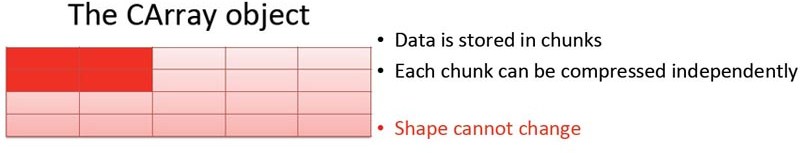
When creating a new CArray (Compressible Array), type and shape must be passed to the constructor:
f = tb.open_file('temp/ctest.h5', 'w')
f.create_carray(f.root, 'my_carray1', tb.Float64Atom(), (10000,1000))
/my_carray1 (CArray(10000, 1000)) ''
  atom := Float64Atom(shape=(), dflt=0.0)
  maindim := 0
  flavor := 'numpy'
  byteorder := 'little'
  chunkshape := (16, 1000)
f.flush()
Now check the temp/ctest.h5 filesize: it's 1KB even if the array is Float64 10000x1000. This is because PyTables just stored the CArray metadata. Now we'll push some data in the CArray container. For simplicity we define a new name for the carray handle: ca = f.root.my_carray1
ca = f.root.my_carray1
na = np.linspace(0, 1, int(1e7)).reshape(10000,1000)
%time ca[:] = na
CPU times: user 16 ms, sys: 32 ms, total: 48 ms
Wall time: 47.3 ms
f.close()
Now check the temp/catest.h5 filesize: it's 76MB whis is exactly the uncompressed space required by a 64bit 10000x1000 matrix.
CArray allows for data compression: lets try to use a blosc compressor with complevel=5: filesize must be reduced to 8.7MB!
f = tb.open_file('temp/ctest.h5', 'w')
f.create_carray(f.root, 'my_carray1', tb.Float64Atom(), (10000,1000),
               filters=tb.Filters(complevel=5, complib='blosc'))
%time f.root.my_carray1[:] = na
f.close()
CPU times: user 216 ms, sys: 20 ms, total: 236 ms
Wall time: 233 ms
*Try by yourself* the following compression options:
(complevel=9, complib='blosc')
(complevel=5, complib='zlib')
(complevel=9, complib='lzo')
(complevel=5, complib='bzip2')
We can now check how much do it takes to read a small, non-contiguous sub-array by using the %timeit magic function: the read operation will be run multiple times to better measure the execution time:
f = tb.open_file('temp/ctest.h5', 'r')
%timeit f.root.my_carray1[:4,::100]
f.close()
45.2 µs ± 1.34 µs per loop (mean ± std. dev. of 7 runs, 10000 loops each)
3 The Table Object
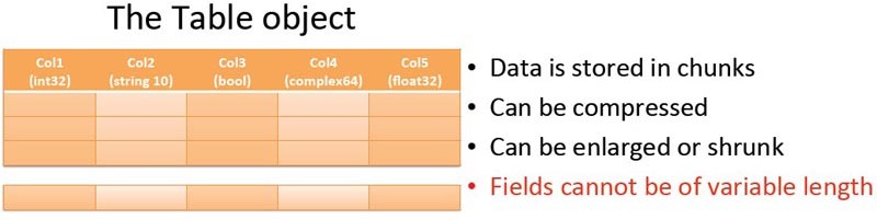
To create a new Table Object we must first describe the fields:
class TabularData(tb.IsDescription):
    col1 = tb.StringCol(200)
    col2 = tb.IntCol()
    col3 = tb.Float32Col(10)
# Open a file and create the Table container
f = tb.open_file('temp/atable.h5', 'w')
t = f.create_table(f.root, 'my_table1', TabularData, 'Table Title',
                  filters=tb.Filters(complevel=5, complib='blosc'))
t
/my_table1 (Table(0,), shuffle, blosc(5)) 'Table Title'
  description := {
  "col1": StringCol(itemsize=200, shape=(), dflt=b'', pos=0),
  "col2": Int32Col(shape=(), dflt=0, pos=1),
  "col3": Float32Col(shape=(10,), dflt=0.0, pos=2)}
  byteorder := 'little'
  chunkshape := (268,)
#  Fill the table with some 1 million rows
from time import time
t0 = time()
r = t.row
for i in range(1000*1000):
    r['col1'] = str(i)
    r['col2'] = i+1
    r['col3'] = np.arange(10, dtype=np.float32)+i
    r.append()
t.flush()
print ("Insert time: {:.3f}s".format(time()-t0,))
Insert time: 3.518s
t
/my_table1 (Table(1000000,), shuffle, blosc(5)) 'Table Title'
  description := {
  "col1": StringCol(itemsize=200, shape=(), dflt=b'', pos=0),
  "col2": Int32Col(shape=(), dflt=0, pos=1),
  "col3": Float32Col(shape=(10,), dflt=0.0, pos=2)}
  byteorder := 'little'
  chunkshape := (268,)
chunkshape := (268,) means that every 268 rows a datachunk is created, compressed and saved on disk.
The uncompressed size of the dataset can be calculated by multiplying the number of rows t.shape[0] by the size of each row t.dtype.itemsize. In this example the size of each row is 244 bytes: 200 bytes for the string field, 4 for the Int field and 40 for the ten Float32. If you check the filesize on disk you will see that since we used a blosc compression algorithm, we managed to reduce the filesize from 232MB to 3.6MB!
t.shape[0]*t.dtype.itemsize/2**20.
232.696533203125
With Tables we can do queries. For example here we extract values of col1 where col2 < 10: in less than one second we query 1.000.000 records.
%time [r['col1'] for r in t if r['col2'] < 10]
CPU times: user 168 ms, sys: 0 ns, total: 168 ms
Wall time: 165 ms
[b'0', b'1', b'2', b'3', b'4', b'5', b'6', b'7', b'8']
We can be even faster by using in-kernel methods instead of using the regular Python condition. Condition defined as a string with the where method are evaluated. numexpr is a package that accepts the expression as a string, analyzes it, rewrites it more efficiently, and compiles it on the fly into code suitable to its internal virtual machine (VM). Due to its integrated just-in-time (JIT) compiler, it does not require a compiler at runtime:
# Repeat the query, but using in-kernel method
%time [r['col1'] for r in t.where('col2 < 10')]
CPU times: user 160 ms, sys: 20 ms, total: 180 ms
Wall time: 158 ms
[b'0', b'1', b'2', b'3', b'4', b'5', b'6', b'7', b'8']
Alternatively, to reach even greater performances, the Table Object support indexing for every column. We can index the colum two:
%time t.cols.col2.create_csindex()
CPU times: user 396 ms, sys: 12 ms, total: 408 ms
Wall time: 407 ms
1000000
From now on, any query involving col2 will be sped-up many times. In this case we query the whole 1.000.000 records in less than 200us (0.0002s):
%timeit [r['col1'] for r in t.where('col2 < 10')]
71.9 µs ± 107 ns per loop (mean ± std. dev. of 7 runs, 10000 loops each)
Queries can involve both indexed and non-indexed colums, in this case the speed-up will be less noticeable. here we do the query in few seconds because col3 is not indexed:
# Performing complex conditions (regular query)
%time [r['col1'] for r in t if r['col2'] > 10 and r['col3'][0] < 20]
CPU times: user 1.93 s, sys: 12 ms, total: 1.94 s
Wall time: 1.93 s
[b'10', b'11', b'12', b'13', b'14', b'15', b'16', b'17', b'18', b'19']
f.close()
4 The EArray Object
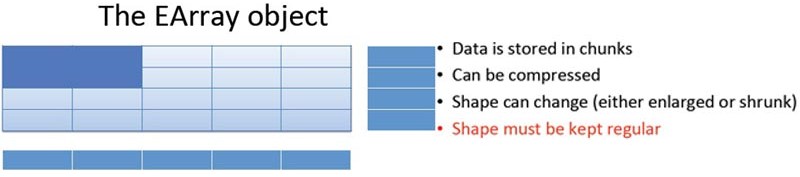
We will illustrate how to use the PyTables EArray (Extensible Array) Object by performing an Out-of-Core calculation. PyTables leverages numexpr to perform computations with arrays that are on disk and not in memory (Out-of-Core). Numexpr performs the computation on large arrays by splitting the arrays in smaller blocks of data, those blocks are then uploaded to the CPU cache memory and the computations are done without macking data copies on RAM
import numpy as np
import tables as tb
f = tb.open_file('temp/poly1.h5', 'w')
Create an empty EArray then populate it with 10 chuncks of 1.000.000 values, we'll have an array with 1 Column and 10.000.000 Rows. In the createEArray method we define the dimension along which the EArray can be expanded. For example, in this case whe define by using (0,) that the array will be expanded along the row dimension. Similarly, if we wanted to expand it by columns, we would use (,0).
ea = f.create_earray(f.root, 'my_earray1', tb.Float64Atom(), (0,),
                    filters=tb.Filters(complevel=5, complib='blosc'))
for s in range(10):
    ea.append(np.linspace(s, s+1, int(1e6)))
ea.flush()
Create the expression to compute: this expression must be defined as a string. Basically, for each row the polynomial will be calculated:
expr = tb.Expr('0.25*ea**3 + 0.75*ea**2 + 1.5*ea - 2')
Now we have to create an array to store the resulting values, in this case we can decide to use a Compressed Array (CArray) with the same lenght of the EArray: 10.000.000 rows
if hasattr(f.root, 'output_values'):
    f.removeNode(f.root.y)
y = f.create_carray(f.root, 'output_values', tb.Float64Atom(), (len(ea),),
                   filters=tb.Filters(complevel=5, complib='blosc'))
Specify that the ouput of the expression has to go to y on disk
expr.set_output(y)
On a standard PC this will take less than a second. This time is significant if you think that data are loaded and stored directly on disk while doing calculation:
%time expr.eval()
CPU times: user 260 ms, sys: 36 ms, total: 296 ms
Wall time: 197 ms
/output_values (CArray(10000000,), shuffle, blosc(5)) ''
  atom := Float64Atom(shape=(), dflt=0.0)
  maindim := 0
  flavor := 'numpy'
  byteorder := 'little'
  chunkshape := (16384,)
f.flush()
Visit www.add-for.com for more tutorials and updates.
This work is licensed under a Creative Commons Attribution-ShareAlike 4.0 International License.