Churn Prediction (Statistical Testing, Stacking Ensemble)

Table of Contents
- 1. Introduction
- 2. Libraries & Configurations
- 3 Descriptive Analysis
- 4 Data Wrangling
- 5 Univariate Analysis
- 6 Bivariate Analysis
- 7 Multivariate Analysis
- 8 Feature Engineering
- 9 Data Preparation
- 10 Modeling
- 11 Conclusions
- 12 References
1 Introduction
The objective of this notebook is to present an extensive analysis of the IBM Customer Churn Dataset and to predict the customer churn rate.
Dataset Source :
GitHub Project Repository :
NB: This project also serves as my assignments for the courses below -
You can also view this notebook on kaggle
1.1 Insights & Summary
- Dataset mostly has categorical variables
- Data is not normally distributed, performed Nonparametric Statistical tests
- Performed statistical hypothesis test to check correlation , multicollinearity
- Imbalanced dataset, did experiment with different sampling techniques(e.g stratifying, imblearn - SMOTE etc)
- Tuned Hyperparameters using Optuna
- All statistical tests were performed with a 95% confidence level (i.e., p value < 0.05)
- Performed single level Stacking Ensemble with Triple Gradient boosting algorithms
2 Libraries & Configurations
2.1 Import Libraries
!pip install --upgrade scipy # to calculate Cramer's V latest version of scipy needed
"""Import basic modules."""
import math
import os
import gc
import random
import pprint
import numpy as np               # For linear algebra
import pandas as pd              # For data manipulation
import matplotlib.pyplot as plt  # For 2D visualization
import seaborn as sns

# Warning Libraries
import warnings
warnings.filterwarnings("ignore")
# warnings.simplefilter(action='ignore', category=FutureWarning)

from collections import Counter
from scipy import stats                         # For statistics
from scipy.stats.contingency import association # upgrade scipy to use this to calculate Cramer's V

"""Plotly visualization"""
import plotly.graph_objs as go
import plotly.express as px
import plotly.io as pio
from plotly.subplots import make_subplots
from plotly.offline import init_notebook_mode, iplot


from sklearn.preprocessing import OrdinalEncoder, OneHotEncoder, LabelEncoder, StandardScaler, MinMaxScaler, RobustScaler, MaxAbsScaler
from sklearn.preprocessing import PowerTransformer # convert to Gaussian-like data
from sklearn.feature_selection import SelectKBest, f_classif, chi2

from sklearn.model_selection import StratifiedShuffleSplit, StratifiedKFold, RepeatedStratifiedKFold, train_test_split, cross_val_score
from sklearn.pipeline import Pipeline, make_pipeline

from imblearn.over_sampling import SMOTE
from imblearn.under_sampling import RandomUnderSampler

# Algorithms
from sklearn.ensemble import StackingClassifier, RandomForestClassifier, ExtraTreesClassifier
from sklearn.linear_model import LogisticRegression
from sklearn.neighbors import KNeighborsClassifier
from sklearn.svm import SVC

# Boosting Algorithms
!pip install catboost
from xgboost                          import XGBClassifier
from catboost                         import CatBoostClassifier, Pool
from lightgbm                         import LGBMClassifier

!pip install optuna
import optuna
from optuna.visualization import plot_optimization_history, plot_param_importances

import multiprocessing
import pickle, joblib
from sklearn.metrics import matthews_corrcoef, roc_auc_score, precision_recall_curve, confusion_matrix, classification_report, roc_curve, auc

from sklearn.utils import resample
from IPython.display import Markdown, display

# utility function to print markdown string
def printmd(string):
    display(Markdown(string))

# customize as needed
plt_params = {
    # 'figure.facecolor': 'white',
    'axes.facecolor' : 'white',

    ## to set size
    # 'legend.fontsize': 'x-large',
    # 'figure.figsize': (15, 10),
    # 'axes.labelsize': 'x-large',
    # 'axes.titlesize': 'x-large',
    # 'xtick.labelsize': 'x-large',
    # 'ytick.labelsize': 'x-large'
}

plt.rcParams.update(plt_params)

sns.set_style('whitegrid')

# init_notebook_mode(connected=True)
# pio.renderers.default='notebook' # to display plotly graph
%matplotlib inline
Check Version
!pip freeze | grep optuna
!pip freeze | grep xgboost
!pip freeze | grep catboost
!pip freeze | grep lightgbm
!pip freeze | grep plotly
!pip freeze | grep scipy
!pip freeze | grep scikit-learn
2.2 Configurations
# padding value
left_padding = 21

# seed value
SEED = 42

# set optuna verbosity level
optuna_verbosity = optuna.logging.WARNING # https://optuna.readthedocs.io/en/latest/reference/logging.html#module-optuna.logging

def seed_everything(seed=42):
    random.seed(seed)
    os.environ['PYTHONHASHSEED'] = str(seed)
    np.random.seed(seed)

seed_everything(SEED)
3 Descriptive Analysis
| Feature Name | Description | Data Type |
|---|---|---|
| customerID | Contains customer ID | categorical |
| gender | whether the customer female or male | categorical |
| SeniorCitizen | Whether the customer is a senior citizen or not (1, 0) | numeric, int |
| Partner | Whether the customer has a partner or not (Yes, No) | categorical |
| Dependents | Whether the customer has dependents or not (Yes, No) | categorical |
| tenure | Number of months the customer has stayed with the company | numeric, int |
| PhoneService | Whether the customer has a phone service or not (Yes, No) | categorical |
| MultipleLines | Whether the customer has multiple lines r not (Yes, No, No phone service) | categorical |
| InternetService | Customer’s internet service provider (DSL, Fiber optic, No) | categorical |
| OnlineSecurity | Whether the customer has online security or not (Yes, No, No internet service) | categorical |
| OnlineBackup | Whether the customer has online backup or not (Yes, No, No internet service) | categorical |
| DeviceProtection | Whether the customer has device protection or not (Yes, No, No internet service) | categorical |
| TechSupport | Whether the customer has tech support or not (Yes, No, No internet service) | categorical |
| streamingTV | Whether the customer has streaming TV or not (Yes, No, No internet service) | categorical |
| streamingMovies | Whether the customer has streaming movies or not (Yes, No, No internet service) | categorical |
| Contract | The contract term of the customer (Month-to-month, One year, Two year) | categorical |
| PaperlessBilling | Whether the customer has paperless billing or not (Yes, No) | categorical |
| PaymentMethod | The customer’s payment method (Electronic check, Mailed check, Bank transfer, Credit card) | categorical |
| MonthlyCharges | The amount charged to the customer monthly | numeric , int |
| TotalCharges | The total amount charged to the customer | object |
| Churn | Whether the customer churned or not (Yes or No) | categorical |
df_churn = pd.read_csv("https://raw.githubusercontent.com/IBM/telco-customer-churn-on-icp4d/master/data/Telco-Customer-Churn.csv")
df_churn.head()
print(f"Dataset Dimension: {df_churn.shape[0]} rows, {df_churn.shape[1]} columns")
df_churn.info()

printmd("<br>**SeniorCitizen** is already converted to ineteger<br><br>**TotalCharges** should be converted to float")
Drop customerID column
del df_churn["customerID"]
3.1 Summary of Categorical Features
df_churn.describe(include=['object']).T
3.2 Checking Duplicates
print('Known observations: {}\nUnique observations: {}'.format(len(df_churn.index),len(df_churn.drop_duplicates().index)))

printmd("**No duplicates Found!**")
3.3 Unique Values
printmd("**Unique Values By Features**")
for feature in df_churn.columns:
    uniq = np.unique(df_churn[feature])
    print(feature.ljust(left_padding),len(uniq))
4 Data Wrangling
4.1 Missing Values
df_churn.isna().sum()
cat_cols = set(df_churn.columns) - set(df_churn._get_numeric_data().columns)

printmd("'**isna**' is only applicable for numerical data type<br>")
printmd("Checking missing values for object data type<br><br>")

for cat in cat_cols:
  print(cat.ljust(left_padding), df_churn[cat].apply(lambda x:len(x.strip()) == 0 or x.strip().lower() == 'nan').sum())

printmd("<br>TotalCharges is an object datatype, it has **11** 'nan' value")
4.1.1 Change Data Type
Convert TotalCharges to numeric
df_churn["TotalCharges"] = pd.to_numeric(df_churn["TotalCharges"], errors = 'coerce')
4.1.2 Imputation
indices_null_tc = df_churn[df_churn["TotalCharges"].isna()].index
display(df_churn.iloc[indices_null_tc])

printmd("<br>**'Tenure' (months stayed at the company) is correlated with 'TotalCharges' column**")
printmd("**when 'Tenure' is 0 , 'TotalCharges' is 0 too**")
display(df_churn[df_churn.tenure == 1].head(2))

printmd("<br>**'TotalCharges' is the same as 'MonthlyCharges' when 'Tenure' is not 0**")
display(df_churn[df_churn.tenure == 3].head(2))

printmd("<br>**'TotalCharges' increases with respect to 'MonthlyCharges' and 'Tenure'**")
printmd("<br>From the above observation we can conclude that, **'TotalCharges'  = 'MonthlyCharges' x 'Tenure' + Extra Cost**")
printmd("**Therefore, imputing missing values on 'TotalCharges' column with 0**")
df_churn['TotalCharges'].fillna(0, inplace=True)
df_churn[['tenure', 'MonthlyCharges', 'TotalCharges']].describe().T
4.2 Binning
There are three numerical data types which can be ranked based on their values :
- Tenure, MonthlyCharges and TotalCharges
We can bin them into three levels : high, medium and low
def binning_feature(feature):
  plt.hist(df_churn[feature])

  # set x/y labels and plot title
  plt.xlabel(f"{feature.title()}")
  plt.ylabel("Count")
  plt.title(f"{feature.title()} Bins")
  plt.show()

  bins = np.linspace(min(df_churn[feature]), max(df_churn[feature]), 4)
  printmd("**Value Range**")

  printmd(f"Low ({bins[0] : .2f} - {bins[1]: .2f})")
  printmd(f"Medium ({bins[1]: .2f} - {bins[2]: .2f})")
  printmd(f"High ({bins[2]: .2f} - {bins[3]: .2f})")
  group_names = ['Low', 'Medium', 'High']

  df_churn.insert(df_churn.shape[1]-1,f'{feature}-binned', pd.cut(df_churn[feature], bins, labels=group_names, include_lowest=True))
  display(df_churn[[feature, f'{feature}-binned']].head(10))


  # count values
  printmd("<br>**Binning Distribution**<br>")
  display(df_churn[f'{feature}-binned'].value_counts())


  # plot the distribution of each bin
  plt.bar(group_names, df_churn[f'{feature}-binned'].value_counts())
  # px.bar(data_canada, x='year', y='pop')

  # set x/y labels and plot title
  plt.xlabel(f"{feature.title()}")
  plt.ylabel("Count")
  plt.title(f"{feature.title()} Bins")
  plt.show()
4.2.1 Tenure
binning_feature('tenure')


4.2.2 MonthlyCharges
binning_feature('MonthlyCharges')


4.2.3 TotalCharges
binning_feature('TotalCharges')


Data Types Distribution after cleaning
printmd("**Data Types**<br>")
df_churn.dtypes.value_counts()
5 Univariate Analysis
5.1 Statistical Normality Tests
Normality tests are used to determine if a dataset is normally distributed and to check how likely it is for a random variable in the dataset to be normally distributed.
Popular normality tests - D’Agostino’s K^2, Shapiro-Wilk, Anderson-Darling .
There are three numerical features in this dataset - MonthlyCharges, Tenure, and TotalCharges.
Hypotheses -
- H0: the sample has a Gaussian distribution.
- H1: the sample does not have a Gaussian distribution.
NB : we can not perform Shapiro-Wilk Test because sample size > 5000 and for this test p-value may not be accurate for N > 5000
5.1.1 D’Agostino’s K^2 Test
MonthlyCharges
stat, p = stats.normaltest(df_churn['MonthlyCharges'])

print('Statistics=%.5f, p=%.3f' % (stat, p))

# interpret
alpha = 0.05
if p > alpha:
	print('Sample looks Gaussian (fail to reject H0)')
else:
	print('Sample does not look Gaussian (reject H0)')
Tenure
stat, p = stats.normaltest(df_churn['tenure'])

print('Statistics=%.5f, p=%.3f' % (stat, p))

# interpret
alpha = 0.05
if p > alpha:
	print('Sample looks Gaussian (fail to reject H0)')
else:
	print('Sample does not look Gaussian (reject H0)')
5.1.2 Anderson-Darling Test
Hypotheses -
- H0: the sample has a Gaussian distribution
- H1: the sample does not have a Gaussian distribution
Critical values in a statistical test are a range of pre-defined significance boundaries at which the H0 can be failed to be rejected if the calculated statistic is less than the critical value. \ Rather than just a single p-value, the test returns a critical value for a range of different commonly used significance levels. \ In this case - normal/exponential (15%, 10%, 5%, 2.5%, 1%)
TotalCharges
result = stats.anderson(df_churn['TotalCharges'])

print('Statistic: %.3f' % result.statistic)

p = 0

for i in range(len(result.critical_values)):
	sl, cv = result.significance_level[i], result.critical_values[i]
	if result.statistic < result.critical_values[i]:
		print(f'Significance level {sl:.2f} % : critical value {cv:.3f}, data looks normal (fail to reject H0)')
	else:
		print(f'Significance level {sl:.2f} % : critical value {cv:.3f}, data does not look normal (reject H0)')
5.2 Visualization
Churn (Target) Distribution
fig = px.pie(df_churn['Churn'].value_counts().reset_index().rename(columns={'index':'Type'}), values='Churn', names='Type', title='Churn (Target) Distribution')
fig.update_traces(textposition='inside', textinfo='percent+label')
fig.show()
printmd("### Target distribution is Imbalanced")
OnlineSecurity, OnlineBackup, DeviceProtection, TechSupport
# Create subplots: use 'domain' type for Pie subplot
fig = make_subplots(rows=2, cols=2, specs=[[{'type':'domain'}, {'type':'domain'}],[{'type':'domain'}, {'type':'domain'}]])

fig.add_trace(go.Pie(labels=df_churn['OnlineSecurity'].value_counts().index, values=df_churn['OnlineSecurity'].value_counts().values, name="Online Security"),
              1, 1)
fig.add_trace(go.Pie(labels=df_churn['OnlineBackup'].value_counts().index, values=df_churn['OnlineBackup'].value_counts().values, name="Online Backup"),
              1, 2)
fig.add_trace(go.Pie(labels=df_churn['DeviceProtection'].value_counts().index, values=df_churn['DeviceProtection'].value_counts().values, name="Device Protection"),
              2, 1)
fig.add_trace(go.Pie(labels=df_churn['TechSupport'].value_counts().index, values=df_churn['TechSupport'].value_counts().values, name="Tech Support"),
              2, 2)

# donut-like pie chart
fig.update_traces(hole=.5, hoverinfo="label+percent")

fig.update_layout(

    # Add annotations in the center of the donut pies.
    annotations=[dict(text='Online<br>Security', x=0.195, y=0.85, font_size=20, showarrow=False),
                 dict(text='Online<br>Backup', x=0.805, y=0.84, font_size=20, showarrow=False),
                 dict(text='Device<br>Protection', x=0.185, y=0.18, font_size=20, showarrow=False),
                 dict(text='Tech<br>Support', x=0.805, y=0.18, font_size=20, showarrow=False)])
fig.update_layout(margin=dict(t=0, b=0, l=0, r=0))
fig.show()


printmd("### 'Online Backup', 'Device Protection' and 'Online Security', 'Tech Support' has similar distribution")
PaymentMethod
display(px.pie(df_churn['PaymentMethod'].value_counts().reset_index().rename(columns={'index':'Type'}), values='PaymentMethod', names='Type', title='Payment Method Distribution'))

printmd("#### Most of the customers use E-check")
Gender
sns.catplot(x="gender", kind="count", data=df_churn)
plt.show()

printmd("#### Approximately 50/50 gender ratio")

Dependents
sns.catplot(x="Dependents", kind="count", data=df_churn)
plt.show()

printmd("#### Users who have non-dependents are approximately two times more than users having dependents")

Senior Citizen
sns.catplot(x="SeniorCitizen", kind="count", data=df_churn)
plt.show()

printmd("#### The majority of the users are not Senior Citizen")

Contract
sns.catplot(x="Contract", kind="count", data=df_churn)
plt.show()

printmd("#### Most of the users prefer Month-to-month contract")

PaperlessBilling
sns.catplot(x="PaperlessBilling", kind="count", data=df_churn)
plt.show()

printmd("#### Most of the users prefer paperless billing")

Total Charges
sns.boxplot(x=df_churn["TotalCharges"])
plt.show()

printmd("#### The total charges fall under 4000 for majority of the users")

Numerical Features
"""#1.Create a function to plot histogram and density plot."""
def plot_histogram(feature):
    """Plots histogram and density plot of a variable."""

    # Create subplot object
    fig = make_subplots(
        rows=2,
        cols=1,
        print_grid=False,
    subplot_titles=(f"Distribution of {feature.name} with Histogram", f"Distribution of {feature.name} with Density Plot"))

    # This is a count histogram
    fig.add_trace(
        go.Histogram(
            x = feature,
            hoverinfo="x+y"
        ),
    row=1,col=1)

    # This is a density histogram
    fig.add_trace(
        go.Histogram(
            x = feature,
            hoverinfo="x+y",
            histnorm = "density"
        ),
    row=2,col=1)

    # Update layout
    fig.layout.update(
        height=800,
        width=870,
        hovermode="closest"
        )

    # Update axes
    fig.layout.yaxis1.update(title="<b>Abs Frequency</b>")
    fig.layout.yaxis2.update(title="<b>Density(%)</b>")
    fig.layout.xaxis2.update(title=f"<b>{feature.name}</b>")
    return fig.show()
plot_histogram(df_churn['tenure'])

printmd("**Tenure is U-shaped distributed**")
plot_histogram(df_churn['MonthlyCharges'])

printmd("**MonthlyCharges is heavily skewed**")
plot_histogram(df_churn['TotalCharges'])

printmd("**TotalCharges is reversed J-shaped distributed**")
6 Bivariate Analysis
In this section, I did an extensive statistical analysis with various hypotheses testing based on paired data types like -
- numerical and numerical data
- numerical and ordinal data
- ordinal and ordinal data
- categorical and categorical data
General Hypotheses -
- H0: the two samples are independent
- H1: there is a dependency between the samples
6.1 List Feature Based on Types
# Check cardinality of categorical variables
target_col_filter = df_churn.loc[:, df_churn.columns != 'Churn']


cat_cols = list(set(target_col_filter.columns) - set(target_col_filter._get_numeric_data().columns))
num_cols = list(set(target_col_filter._get_numeric_data().columns) - set({'SeniorCitizen'})) # already converted to integer


# Get number of unique entries in each column with categorical data
object_nunique = list(map(lambda col: target_col_filter[col].nunique(), cat_cols))
dict_features_by_col = dict(zip(cat_cols, object_nunique))


# Print number of unique entries by column, in ascending order
print(sorted(dict_features_by_col.items(), key=lambda x: x[1]))


ordinal_cols = ['tenure-binned', 'MonthlyCharges-binned', 'TotalCharges-binned']
dichotomous_cols = [cat for cat in cat_cols if df_churn[cat].value_counts().count() == 2]
polytomous_cols = list(set(cat_cols) - set(dichotomous_cols) - set(ordinal_cols))


print("Categorical Columns".ljust(left_padding), cat_cols)
print("Numerical Columns".ljust(left_padding), num_cols)
print("Ordinal Columns".ljust(left_padding), ordinal_cols)
print("Dichotomous Columns".ljust(left_padding), dichotomous_cols)
print("Polytomous Columns".ljust(left_padding), polytomous_cols)
Categorical Columns
'TechSupport', 'DeviceProtection', 'Contract', 'PaperlessBilling', 'TotalCharges-binned',
'gender', 'OnlineBackup', 'InternetService', 'StreamingTV', 'tenure-binned',
'Dependents', 'PhoneService', 'StreamingMovies', 'MultipleLines', 'Partner',
'MonthlyCharges-binned', 'OnlineSecurity', 'PaymentMethod'
Numerical Columns
'MonthlyCharges', 'tenure', 'TotalCharges'
Ordinal Columns
tenure-binned', 'MonthlyCharges-binned', 'TotalCharges-binned'
Dichotomous Columns
'PaperlessBilling', 'gender', 'Dependents', 'PhoneService', 'Partner'
Polytomous Columns
'TechSupport', 'StreamingMovies', 'DeviceProtection', 'MultipleLines', 'Contract',
'InternetService', 'OnlineSecurity', 'StreamingTV', 'PaymentMethod', 'OnlineBackup'
6.2 Numerical & Numerical
6.2.1 Spearman rank-order correlation
AKA Spearman's rho or Spearman correlation coefficient\ Applied to Continuous or ordinal
Unlike the Pearson correlation, the Spearman correlation does not assume that both datasets are normally distributed
Pearson correlation assumes normality, linearity and homoscedasticity.Pearson's correlation is also not able to tell the difference between dependent and independent variables
Hypotheses -
- H0: the two samples do not have monotonic relationship
- H1: there is a monotonic relationship between the samples
For Pearson r correlation, both variables should be normally distributed
According to the normality test tenure, MonthlyCharges and TotalCharges columns are not normally distributed
def cal_spearmanr(c1, c2):

  alpha = 0.05

  correlation, p_value = stats.spearmanr(df_churn[c1], df_churn[c2])

  print(f'{c1}, {c2} correlation : {correlation}, p : {p_value}')

  if p_value > alpha:
    print('Probably do not have monotonic relationship (fail to reject H0)')
  else:
    print('Probably have monotonic relationship (reject H0)')
cal_spearmanr('tenure','MonthlyCharges')
cal_spearmanr('tenure','TotalCharges')
cal_spearmanr('MonthlyCharges','TotalCharges')
6.3 Numerical & Categorical
6.3.1 Kendall rank correlation coefficient
AKA Kendall's τ or Kendall's Tau
Kendall’s Tau is often used for correlation on continuous data if there are outliers in the data
A τ test is a non-parametric hypothesis test for statistical dependence based on the τ coefficient
Variable would be continuous or ordinal
Ordinal variable examples -
- age, weight, height, test scores, survey scores, yearly salary, etc
- education level (GDE/Bachelors/Masters/PhD), income level (if grouped into high/medium/low) etc
In this dataset there are three ordinal features :
- tenure-binned
- MonthlyCharges-binned
- TotalCharges-binned
def kendall_rank_correlation(feature1, feature2):

  coef, p_value = stats.kendalltau(df_churn[feature1], df_churn[feature2])
  print(f"Correlation between {feature1} and {feature2} ")
  print('Kendall correlation coefficient = %.5f, p = %.5f' % (coef, p_value))

  # interpret the significance
  alpha = 0.05
  if p_value > alpha:
    print('Samples are uncorrelated (fail to reject H0) p=%.3f' % p_value)
  else:
    print('Samples are correlated (reject H0) p=%.3f' % p_value)
  print('----\n')
ordinal_features = ['tenure-binned','MonthlyCharges-binned', 'TotalCharges-binned']

for ord in ordinal_features:
  printmd(f"Correlation with **{ord}**")
  kendall_rank_correlation('tenure',ord)
  kendall_rank_correlation('MonthlyCharges',ord)
  kendall_rank_correlation('TotalCharges',ord)
6.3.2 Mann-Whitney U Test
The Mann-Whitney U test is a nonparametric statistical significance test for determining whether two independent samples were drawn from a population with the same distribution.
The test determines whether the medians of two or more groups are different.
NB : For the test to be effective, it requires at least 20 observations in each data sample.
- Fail to Reject H0: Sample distributions are equal. (or sample distributions are likely drawn from the same population)
- Reject H0: Sample distributions are not equal.
or
- H0: population medians are equal.
- H1: population medians are not equal.
Correlation with Target (Dichotomous)
def mannwhitneyu_correlation(feature1):
  stat, p_value = stats.mannwhitneyu(df_churn[feature1], (df_churn['Churn'] == 'Yes').astype(int))
  print(f"Correlation between {feature1} and Churn")
  print('Statistics = %.5f, p = %.5f' % (stat, p_value))

  # interpret the significance
  alpha = 0.05
  if p_value > alpha:
      print('Same distribution (fail to reject H0)')
  else:
      print('Different distribution (reject H0)')
  print('----\n')
numerical_features = ['tenure','MonthlyCharges', 'TotalCharges']

for num in numerical_features:
  printmd(f"Correlation with **{num}**")
  mannwhitneyu_correlation(num)
Biserial correlation
The point biserial correlation is used to measure the relationship between a binary variable, x, and a continuous variable, y. Like other correlation coefficients, this one varies between -1 and +1 with 0 implying no correlation. Correlations of -1 or +1 imply a determinative relationship.
NB: point-biserial correlation is conducted with the Pearson correlation formula except that one of the variables is dichotomous
The assumptions for Point-Biserial correlation include:
- Continuous and Binary
- Normally Distributed (In our case not normal)
- No Outliers
- Equal Variances
Options to normalize a non-normal distribution -
- Log transform
- Square root transform
- Box cox (can only be applied to strictly positive data)
- Yeo Johnson (both positive and negative)
# https://stackoverflow.com/questions/53624804/how-to-normalize-a-non-normal-distribution

data = df_churn['MonthlyCharges'].to_numpy()
pt = PowerTransformer(method='yeo-johnson') # ‘box-cox’, 'yeo-johnson'
data = data.reshape(-1, 1)
pt.fit(data)
transformed_data = pt.transform(data)

transformed_k2, transformed_p = stats.normaltest(transformed_data)

# other methods to transform into gaussian distribution

# stats.normaltest(np.log(df_churn['MonthlyCharges']))
# stats.normaltest(np.sqrt(df_churn['MonthlyCharges'])
# stats.normaltest(stats.boxcox(df_churn['MonthlyCharges'])[0])

# all other methods failed to convert into gaussian


alpha = 0.05
if transformed_p > alpha:
	print('Sample looks Gaussian (fail to reject H0)')
else:
	print('Sample does not look Gaussian (reject H0)')
Since the numerical columns can not be converted to gaussian distribution, point biseral correlation test can not be performed
6.3.3 Polytomous(Nominal) with numeric
For a dichotomous categorical variable and a continuous variable we can calculate a Pearson correlation if the categorical variable has a 0/1-coding for the categories. This correlation is then also known as a point-biserial correlation coefficient. (parametric test)
But when we have more than two categories for the categorical variable the Pearson correlation is not appropriate anymore. \ We should then use eta-squared, or eta, as an effect-size measure for the relationship of a categorical variable and a continuous variable.
def correlation_ratio(categories, measurements):
    fcat, _ = pd.factorize(categories)
    cat_num = np.max(fcat)+1
    y_avg_array = np.zeros(cat_num)
    n_array = np.zeros(cat_num)
    for i in range(0,cat_num):
        cat_measures = measurements[np.argwhere(fcat == i).flatten()]
        n_array[i] = len(cat_measures)
        y_avg_array[i] = np.average(cat_measures)
    y_total_avg = np.sum(np.multiply(y_avg_array,n_array))/np.sum(n_array)
    numerator = np.sum(np.multiply(n_array,np.power(np.subtract(y_avg_array,y_total_avg),2)))
    denominator = np.sum(np.power(np.subtract(measurements,y_total_avg),2))
    if numerator == 0:
        eta = 0.0
    else:
        eta = np.sqrt(numerator/denominator)
    return eta
correlation_ratio(df_churn['PaymentMethod'], df_churn['MonthlyCharges'])
correlation_ratio(df_churn['PaymentMethod'], df_churn['TotalCharges'])
correlation_ratio(df_churn['PaymentMethod'], df_churn['tenure'])
6.4 Dichotomous & Dichotomous
In classification, when both of them are categorical, then the strength of the relationship between them can be measured using a Chi-square test
printmd("**Correlation Between Dichotomous Features with Target : Churn**")

for col in dichotomous_cols:
  print(col.ljust(left_padding), matthews_corrcoef(df_churn[col], df_churn['Churn']))
6.5 Categorical & categorical
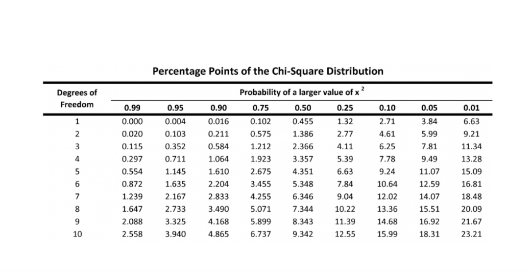
6.5.1 Chi-Square
detect independence between 2 categorical variables, 2x2 or 2xMany
Test statistic in the context of the chi-squared distribution with the requisite number of degrees of freedom
- If Statistic >= Critical Value: significant result, reject null hypothesis (H0), dependent.
- If Statistic < Critical Value: not significant result, fail to reject null hypothesis (H0), independent.
In terms of a p-value and a chosen significance level (alpha):
- If p-value <= alpha: significant result, reject null hypothesis (H0), dependent.
- If p-value > alpha: not significant result, fail to reject null hypothesis (H0), independent
# alpha/significance = 0.05
# If p-value <= alpha: significant result, reject null hypothesis (H0), dependent
# If p-value > alpha: not significant result, fail to reject null hypothesis (H0), independent

def calculate_chi_square(feature1, feature2='Churn'):
  printmd(f"Correlation between **{feature1}** and **{feature2}**")
  crosstab = pd.crosstab(df_churn[feature1], df_churn[feature2])
  # display(crosstab)
  stat, p, dof, expected = stats.chi2_contingency(crosstab,correction=True)


  print(f'p-value : {p}, degree of freedom: {dof}')
  # print("expected frequencies :\n", expected)

  # interpret test-statistic
  prob = 0.95
  critical = stats.chi2.ppf(prob, dof)
  print('probability=%.3f, critical=%.3f, stat=%.3f' % (prob, critical, stat))

  if abs(stat) >= critical:
    print('Dependent (reject H0)')
  else:
    print('Independent (fail to reject H0)')

  # interpret p-value
  alpha = 1.0 - prob

  print('significance=%.3f, p=%.3f' % (alpha, p))
  if p <= alpha:
    print('Dependent (reject H0)')
  else:
    print('Independent (fail to reject H0)')
  print('-----------------------------------\n')

# credit : https://machinelearningmastery.com/chi-squared-test-for-machine-learning
Dichotomous Features
printmd("**Chi-Squre Correlation Between Dichotomous Features with Target : Churn**")

for col in dichotomous_cols:
  calculate_chi_square(col)
With 5% significance level 'PhoneService' and 'gender' features are not dependent with the target : Churn
Polytomous Features
printmd("**Chi-Squre Correlation Between Polytomous Features with Target : Churn**")

for col in polytomous_cols:
  calculate_chi_square(col)
With 5% significance level All polytomous features are dependent with the target : Churn
6.5.2 Cramér’s V
It is based on a nominal variation of Pearson’s Chi-Square Test\ Like correlation, Cramer’s V is symmetrical — it is insensitive to swapping x and y
Cramer's V is used to examine the association between two categorical variables when there is more than a 2 X 2 contingency (e.g., 2 X 3).\ In these more complicated designs, phi correlation test is not appropriate, but Cramer's statistic is. Cramer's V represents the association or correlation between two variables. This statistic is also referred to as "Cramers Phi"
To know more about this, visit this article : the-search-for-categorical-correlation
def cramers_v(x, y):
  """ calculate Cramers V statistic for categorial-categorial association.
      uses correction from Bergsma and Wicher,
      Journal of the Korean Statistical Society 42 (2013): 323-328
  """
  confusion_matrix = pd.crosstab(x,y)
  chi2 = stats.chi2_contingency(confusion_matrix)[0]
  n = confusion_matrix.sum().sum()
  phi2 = chi2/n
  r,k = confusion_matrix.shape
  phi2corr = max(0, phi2-((k-1)*(r-1))/(n-1))
  rcorr = r-((r-1)**2)/(n-1)
  kcorr = k-((k-1)**2)/(n-1)
  return np.sqrt(phi2corr/min((kcorr-1),(rcorr-1)))

# credit : https://stackoverflow.com/a/46498792/11105356
printmd("**Correlation Between Polytomous Features with Target : Churn**")
cramer_v_val_dict = {}
for col in polytomous_cols:
  cramer_v_val_dict[col] = cramers_v(df_churn[col], df_churn['Churn'])

cramer_v_val_dict_sorted = sorted(cramer_v_val_dict.items(), key=lambda x:x[1], reverse=True)

for k,v in cramer_v_val_dict_sorted:
  print(k.ljust(left_padding), v)

printmd("<br>**Contract, OnlineSecurity, TechSupport, InternetService are moderately correlated with Churn**<br>")
printmd("**Cramers V Heatmap on Polytomous Features and Target: Churn**")
cramers_v_val = pd.DataFrame(index=['Churn'], columns=polytomous_cols)

for j in range(0,len(polytomous_cols)):
  u = cramers_v(df_churn['Churn'], df_churn[polytomous_cols[j]])
  cramers_v_val.loc[:,polytomous_cols[j]] = u

cramers_v_val.fillna(value=np.nan,inplace=True)
plt.figure(figsize=(20,1))
sns.heatmap(cramers_v_val,annot=True,fmt='.3f', cmap="YlGnBu")
plt.show()

Using Scipy Module
crosstab = pd.crosstab(df_churn['OnlineSecurity'], df_churn['Churn'])
display(crosstab)
printmd(f"Association between OnlineSecurity and Target:Churn **{stats.contingency.association(crosstab, method='cramer')}**")
6.5.3 Uncertainty Coefficient
AKA Theil’s U - an asymmetric measure of association between categorical features
It is is based on the conditional entropy between x and y — or in human language, given the value of x, how many possible states does y have, and how often do they occur.
Formaly marked as U(x|y); Just like Cramer’s V, the output value is on the range of [0,1], where 0 means that feature y provides no information about feature x, and 1 means that feature y provides full information about features x's value
Unlike Cramer’s V, it is asymmetric
So we will not lose any valuable information unlike symmetric tests
def conditional_entropy(x,y):
  # entropy of x given y
  y_counter = Counter(y)
  xy_counter = Counter(list(zip(x,y)))
  total_occurrences = sum(y_counter.values())
  entropy = 0
  for xy in xy_counter.keys():
      p_xy = xy_counter[xy] / total_occurrences
      p_y = y_counter[xy[1]] / total_occurrences
      entropy += p_xy * math.log(p_y/p_xy)
  return entropy

def theil_u(x,y):
  s_xy = conditional_entropy(x,y)
  x_counter = Counter(x)
  total_occurrences = sum(x_counter.values())
  p_x = list(map(lambda n: n/total_occurrences, x_counter.values()))
  s_x = stats.entropy(p_x)
  if s_x == 0:
      return 1
  else:
      return (s_x - s_xy) / s_x
theilu = pd.DataFrame(index=['Churn'], columns=cat_cols)

for j in range(0,len(cat_cols)):
  u = theil_u(df_churn['Churn'].tolist(),df_churn[cat_cols[j]].tolist())
  theilu.loc[:,cat_cols[j]] = u

theilu.fillna(value=np.nan,inplace=True)
plt.figure(figsize=(20,1))
sns.heatmap(theilu,annot=True,fmt='.2f')
plt.show()

printmd("**Contract, OnlineSecurity, TechSupport, tenure-binned are moderately correlated with Churn**")

6.6 Collinearity
For categorical variables, multicollinearity can be detected with Spearman rank correlation coefficient (ordinal variables) and chi-square test (nominal variables)
For categorical and a continuous variable, multicollinearity can be measured by t-test (if the categorical variable has 2 categories, parametric) or ANOVA (more than 2 categories, parametric)
Spearman's ρ was already performed, proceeding with chi-square
6.6.1 Chi-Square
calculate_chi_square('PaymentMethod','MultipleLines')
calculate_chi_square('PaymentMethod','PhoneService')
calculate_chi_square('PaymentMethod','Contract')
6.7 Visualization
Tenure and MonthlyCharges Distribution
plt.figure(figsize=(10,6),dpi=100)
sns.kdeplot(df_churn.tenure, color='b', shade=True, Label='Tenure')
sns.kdeplot(df_churn.MonthlyCharges, color='r', shade=True, Label='Monthly Charges')

plt.xlabel('Tenure vs Monthly Charges')
plt.ylabel('Probability Density')
plt.legend()
plt.show()

printmd("""**Both are are not normally distributed, skewed,Tenure has a
Bi-modal distribution <br>Most users stayed for less than 20 months,
Monthly Charges for most people is nearly 20 unit**""")

# https://stackoverflow.com/a/65242391/11105356

df_g = df_churn.groupby(['StreamingTV', 'Churn']).size().reset_index()
df_g['percentage'] = df_churn.groupby(['StreamingTV', 'Churn']).size().groupby(level=0).apply(lambda x: 100 * x / float(x.sum())).values
df_g.columns = ['StreamingTV', 'Churn', 'Counts', 'Percentage']

fig = px.bar(df_g, x='StreamingTV', y='Counts',
       color='Churn',
       color_discrete_map={
        'Yes': '#99D594',
        'No': '#FC8D59',
    },
    text=df_g['Percentage'].apply(lambda x: '{0:1.2f}%'.format(x)))

display(fig)
printmd("**Similar ratio between streamer vs non-streamer in churned users**")
Contract and Churn
sns.set(rc={'figure.figsize':(15,8)})
ax=sns.countplot(x='Contract',hue='Churn',data=df_churn)
for p in ax.patches:
    patch_height = p.get_height()
    if np.isnan(patch_height):
        patch_height = 0
    ax.annotate('{}'.format(int(patch_height)), (p.get_x()+0.05, patch_height+10))
plt.show()

printmd("**Most churned users has Month-to-month contract**")

OnlineSecurity and Churn
sns.set(rc={'figure.figsize':(15,8)})
ax=sns.countplot(x='OnlineSecurity',hue='Churn',data=df_churn)
for p in ax.patches:
    patch_height = p.get_height()
    if np.isnan(patch_height):
        patch_height = 0
    ax.annotate('{}'.format(int(patch_height)), (p.get_x()+0.05, patch_height+10))
plt.show()

printmd("**Most churned users didn't have online security**")

Partner and Churn
sns.catplot(x='Partner',hue='Churn',data=df_churn, kind="count");

printmd("**Most users who churned does not have a partner in contrast to the users who does**")

Gender, TotalCharges and Churn
sns.catplot(x='Churn',y='TotalCharges', col = 'gender', data=df_churn,
                kind='bar', aspect=.6, palette='Set2')

printmd("**Gender is uncorrelated with churn rate**")

Checking Outliers
px.box(df_churn, x="Churn", y="MonthlyCharges")
px.box(df_churn, x="Churn", y="TotalCharges")
px.box(df_churn, x="Churn", y="tenure")
plt.figure(figsize=(15,8))
ax = sns.boxplot(x="PaymentMethod", y="TotalCharges", data=df_churn)
plt.show()

printmd("**Total Charges for many users are in extreme level in Mailed Check payment method**")

plt.figure(figsize=(15,8))
ax = sns.boxplot(x="PaymentMethod", y="MonthlyCharges", data=df_churn)
plt.show()

7 Multivariate Analysis
7.1 Multicollinearity (Kruskal–Wallis)
The test is more commonly used when we have three or more levels. For two levels, the Mann Whitney U Test is appropriate
The parametric equivalent of the Kruskal–Wallis test is the one-way analysis of variance (ANOVA)
Hypothses -
- Fail to Reject H0: All sample distributions are equal.
- Reject H0: One or more sample distributions are not equal.
# compare samples
stat, p = stats.kruskal(df_churn['TotalCharges'], df_churn['tenure'], df_churn['MonthlyCharges'])
print('Statistics=%.3f, p=%.3f' % (stat, p))
# interpret
alpha = 0.05
if p > alpha:
	print('Same distributions (fail to reject H0)')
else:
	print('Different distributions (reject H0)')
# compare samples
stat, p = stats.kruskal(df_churn['DeviceProtection'], df_churn['StreamingMovies'], df_churn['PhoneService'])
print('Statistics=%.3f, p=%.3f' % (stat, p))
# interpret
alpha = 0.05
if p > alpha:
	print('Same distributions (fail to reject H0)')
else:
	print('Different distributions (reject H0)')
# compare samples
stat, p = stats.kruskal(df_churn['Contract'], df_churn['PaymentMethod'], df_churn['PhoneService'], df_churn['InternetService'])
print('Statistics=%.3f, p=%.3f' % (stat, p))
# interpret
alpha = 0.05
if p > alpha:
	print('Same distributions (fail to reject H0)')
else:
	print('Different distributions (reject H0)')
7.2 Frequency Distribution
def multivariate_analysis(cat_var_1, cat_var_2, cat_var_3, target_variable=df_churn.Churn):

    fig,ax = plt.subplots(1,1,figsize = (18,5))
    font_size = 15
    cat_grouped_by_cat_target = pd.crosstab(index = [cat_var_1, cat_var_2, cat_var_3],
                                        columns = target_variable, normalize = "index")*100
    cat_grouped_by_cat_target.rename({"Yes":"% Churn", "No":"% Not Churn"}, axis = 1, inplace = True)
    cat_grouped_by_cat_target.plot.bar(color = ["green", "red"],ax=ax)
    ax.set_xlabel(f"{cat_var_1.name}, {cat_var_2.name}, {cat_var_3.name}", fontsize = font_size)
    ax.set_ylabel("Relative Frequency(%)", fontsize = font_size)
    ax.tick_params(axis="x", labelsize=font_size)
    ax.tick_params(axis="y", labelsize=font_size)
    plt.legend(loc = "best")
    return plt.show()
multivariate_analysis(df_churn.Contract, df_churn.InternetService, df_churn.PaymentMethod)
printmd("### Findings: Most of the users who churned had a Month-to-month contract and had internet service")

multivariate_analysis(df_churn.MultipleLines, df_churn['tenure-binned'], df_churn.PhoneService)
printmd("## Findings: Most of the users who churned had phone service")

7.3 Churn Count Distribution
def plot_counting_distribution(cardinality_value):

  #label encoding binary columns
  le = LabelEncoder()

  tmp_churn = df_churn[df_churn['Churn'] == 'Yes']
  tmp_no_churn = df_churn[df_churn['Churn'] == 'No']

  selected_columns = df_churn.nunique()[df_churn.nunique() == cardinality_value].keys()

  for col in selected_columns :
      tmp_churn[col] = le.fit_transform(tmp_churn[col])


  data_frame_x = tmp_churn[selected_columns].sum().reset_index()
  data_frame_x.columns = ["feature","Yes"]
  data_frame_x["No"] = tmp_churn.shape[0]  - data_frame_x["Yes"]
  data_frame_x = data_frame_x[data_frame_x["feature"] != "Churn"]

  #count of 1's(yes)
  trace1 = go.Scatterpolar(r=data_frame_x["Yes"].values.tolist(),
                          theta=data_frame_x["feature"].tolist(),
                          fill="toself", name="Churn 1's",
                          mode="markers+lines", visible=True,
                          marker=dict(size=5)
                          )

  #count of 0's(No)
  trace2 = go.Scatterpolar(r=data_frame_x["No"].values.tolist(),
                          theta=data_frame_x["feature"].tolist(),
                          fill="toself",name="Churn 0's",
                          mode="markers+lines", visible=True,
                          marker=dict(size = 5)
                          )
  for col in selected_columns :
      tmp_no_churn[col] = le.fit_transform(tmp_no_churn[col])

  data_frame_x = tmp_no_churn[selected_columns].sum().reset_index()
  data_frame_x.columns  = ["feature","Yes"]
  data_frame_x["No"]    = tmp_no_churn.shape[0]  - data_frame_x["Yes"]
  data_frame_x  = data_frame_x[data_frame_x["feature"] != "Churn"]

  #count of 1's(yes)
  trace3 = go.Scatterpolar(r = data_frame_x["Yes"].values.tolist(),
                          theta = data_frame_x["feature"].tolist(),
                          fill  = "toself",name = "NoChurn 1's",
                          mode = "markers+lines", visible=False,
                          marker = dict(size = 5)
                          )

  #count of 0's(No)
  trace4 = go.Scatterpolar(r = data_frame_x["No"].values.tolist(),
                          theta = data_frame_x["feature"].tolist(),
                          fill  = "toself",name = "NoChurn 0's",
                          mode = "markers+lines", visible=False,
                          marker = dict(size = 5)
                          )

  data = [trace1, trace2, trace3, trace4]

  updatemenus = list([
      dict(active=0,
          x=-0.15,
          buttons=list([
              dict(
                  label = 'Churn Dist',
                  method = 'update',
                  args = [{'visible': [True, True, False, False]},
                      {'title': f'Customer Churn Binary Counting Distribution' }]),

              dict(
                    label = 'No-Churn Dist',
                  method = 'update',
                  args = [{'visible': [False, False, True, True]},
                      {'title': f'No Customer Churn Binary Counting Distribution'}]),

          ]),
      )
  ])

  layout = dict(title='ScatterPolar Distribution of Churn and Non-Churn Customers (Select from Dropdown)',
                showlegend=False,
                updatemenus=updatemenus)

  fig = dict(data=data, layout=layout)

  pio.show(fig)

# Thanks to : https://www.kaggle.com/kabure/insightful-eda-churn-customers-models-pipeline#Feature-Engineering
7.3.1 Features With Cardinality = 2
plot_counting_distribution(2)
7.3.2 Features With Cardinality = 3
plot_counting_distribution(3)
8 Feature Engineering
For classification generally these methods are used: chi2, f_classif, mutual_info_classif
chi2: Computes chi-squared stats between each non-negative feature and class. This score can be used to select the n_features features with the highest values for the test chi-squared statistic from X, which must contain only non-negative features such as booleans or frequencies (e.g., term counts in document classification), relative to the classes.
f_classif: Compute the ANOVA F-value for the provided sample.
mutual_info_classif: Estimates mutual information for a discrete target variable. Mutual information (MI) between two random variables is a non-negative value, which measures the dependency between the variables. It is equal to zero if and only if two random variables are independent, and higher values mean higher dependency.
source= https://scikit-learn.org/stable/modules/feature_selection.html
N.B : I may apply One Hot Encoding for the categorical columns, But to compare the correlation results obtained from previous notebook with model feature importance I am keeping the feature set as it is ,applying only ordinal encoding
# remove features based on feature importance
# df_churn_cleaned.drop(['gender','Partner','PhoneService','MultipleLines','StreamingMovies'], axis=1, inplace=True)


df_churn_ohe = pd.get_dummies(df_churn_cleaned)

# remove duplicated columns after on hot encoding
df_churn_ohe.drop(['MultipleLines_No phone service',
               'OnlineSecurity_No internet service',
               'OnlineBackup_No internet service',
               'DeviceProtection_No internet service',
               'TechSupport_No internet service',
               'StreamingTV_No internet service',
               'StreamingMovies_No internet service'],axis=1, inplace=True)
8.1 Encode Target variable
df_churn_cleaned = df_churn.copy()
df_churn_cleaned.Churn[df_churn_cleaned.Churn.str.lower() == 'yes'] = 1
df_churn_cleaned.Churn[df_churn_cleaned.Churn.str.lower() == 'no'] = 0

df_churn_cleaned['Churn'] = df_churn_cleaned['Churn'].astype('float')
df_churn_cleaned.to_csv("Telco-Customer-Churn-dataset-cleaned.csv", index=False)
printmd("**Column Info**")
display(df_churn_cleaned.info())
printmd("<br>**Datatypes Count**")
display(df_churn.dtypes.value_counts())
printmd("<br>**Categorical Features**")
display(df_churn.describe(include=['object']).T)
9 Data Preparation
9.1 Prepare Train/Test dataset
strat_split = StratifiedShuffleSplit(n_splits=1, test_size=0.2, random_state=SEED)
for train_index, test_index in strat_split.split(df_churn_cleaned, df_churn_cleaned["Churn"]):
    strat_train_set = df_churn_cleaned.loc[train_index]
    strat_test_set = df_churn_cleaned.loc[test_index]

print('Target Labels Ratio in Original Dataset\n')
print(df_churn_cleaned["Churn"].value_counts(normalize=True).sort_index())
# df_churn_cleaned["Churn"].value_counts() / len(strat_test_set)

print('\nTarget Labels Ratio in Test Dataset\n')
print(strat_test_set["Churn"].value_counts(normalize=True).sort_index())
# strat_test_set["Churn"].value_counts() / len(strat_test_set)
# train Dataset
X = strat_train_set.drop("Churn", axis=1)
y = strat_train_set["Churn"].copy()

# test dataset
y_test = strat_test_set['Churn'].values
X_test = strat_test_set.drop('Churn',axis=1)

X.shape, y.shape, X_test.shape, y_test.shape
# Check cardinality of categorical variables :

# reinitiate cat_cols because 'customerID' is still included in cat_cols variable
cat_cols = list(set(X.columns) - set(X._get_numeric_data().columns))
num_cols = list(set(X._get_numeric_data().columns) - set({'SeniorCitizen'})) # already converted
# Get number of unique entries in each column with categorical data
object_nunique = list(map(lambda col: X[col].nunique(), cat_cols))
d = dict(zip(cat_cols, object_nunique))

print("Number of unique entries by column, in ascending order:\n")
pprint.pprint(sorted(d.items(), key=lambda x: x[1]))

print("Total Categorical Columns",len(cat_cols))
print("Total Numerical Columns",len(num_cols))

printmd("**<br>Dataset has maximum cardinality value of 4 which is comparatively low<br>**")
9.2 Encoding & Scaling
ordinal_encoder = OrdinalEncoder()
X[cat_cols] = ordinal_encoder.fit_transform(X[cat_cols])
X_test[cat_cols] = ordinal_encoder.transform(X_test[cat_cols])

le = LabelEncoder()
y = le.fit_transform(y)

y_test = le.fit_transform(y_test)


num_cols = ['tenure', 'MonthlyCharges', 'TotalCharges']

transformer = RobustScaler()
X[num_cols] = transformer.fit_transform(X[num_cols])
X_test[num_cols] = transformer.transform(X_test[num_cols])
Correlation Heatmap
Pearson’s R (parametric) is not applicable when the data is categorical
Kendall’s Tau is a non-parametric measure of relationships between continuous or ordinal features
While Pearson's correlation assesses linear relationships, Spearman's correlation (non -parametric) assesses monotonic relationships (whether linear or not)
Most of the features in this dataset are categorical and nominal, so it's ineffective for those non-numerical attributes
Moreover, there are only three numerical features which are not normally distributed
Therefore, pandas.corr() is not feasible to use for this case
# Correlation Matrix
# only numerical output
corr_matrix = pd.concat([X[num_cols],strat_train_set[["Churn"]]],axis=1).corr()

# Set Up Mask To Hide Upper Triangle
mask = np.zeros_like(corr_matrix, dtype=np.bool)
mask[np.triu_indices_from(mask)]= True

with sns.axes_style("white"):
    f, ax = plt.subplots(figsize=(7, 5))
    ax = sns.heatmap(corr_matrix,
                      mask = mask,
                      square = True,
                      linewidths = .5,
                      cmap = 'coolwarm',
                      cbar_kws = {'shrink': .4,
                                'ticks' : [-1, -.5, 0, 0.5, 1]},
                      vmin = -1,
                      vmax = 1,
                      annot = True,
                      annot_kws = {'size': 12})

#add the column names as labels
ax.set_yticklabels(corr_matrix.columns, rotation = 0, fontsize=13)
ax.set_xticklabels(corr_matrix.columns, fontsize=13)

sns.set_style({'xtick.bottom': True}, {'ytick.left': True})
plt.show()

printmd("**Tenure is moderately correlated Numerical Feature with Target**")

10 Modeling
10.1 Utility Function
10.1.1 Training
def train_model(model, model_name, X, y, X_test, fold):
  printmd(f'**{model_name} Init**')
  auc_scores = []

  test_preds=None

  strat_kf = StratifiedKFold(n_splits=fold, random_state=SEED, shuffle=True)

  for fold, (train_index, valid_index) in enumerate(strat_kf.split(X, y)):
    X_train, X_valid = X.iloc[train_index] , X.iloc[valid_index]
    y_train, y_valid = y[train_index] , y[valid_index]


    #### to SMOTE sampling
    # sm = SMOTE(sampling_strategy='all', random_state=SEED)
    # X_train_oversampled, y_train_oversampled = sm.fit_resample(X_train, y_train)
    # X_val_oversampled, y_val_oversampled = sm.fit_resample(X_valid, y_valid)

    eval_set = [(X_valid, y_valid)]

    print("-" * 50)
    print(f"Fold {fold + 1}")

    if model_name == 'cat':
      model.fit(X_train, y_train, eval_set= eval_set, verbose=False)
    elif model_name == 'xgb':
      model.fit(X_train, y_train, eval_set= eval_set, eval_metric = 'auc', verbose = False, early_stopping_rounds = 200)
    else:
      model.fit(X_train, y_train, eval_set= eval_set, eval_metric = 'auc', verbose = False, early_stopping_rounds = 200)


    val_pred = model.predict_proba(X_valid)[:,1]
    auc = roc_auc_score(y_valid, val_pred) # AUROC requires probabilities of the predictions
    print("AUC Score : ",auc)

    auc_scores.append(auc)

    if test_preds is None:
      test_preds = model.predict_proba(X_test)[:,1]
    else:
      test_preds += model.predict_proba(X_test)[:,1]


    del X_train, y_train, X_valid, y_valid
    gc.collect()

  print("-" * 50)
  test_preds /= fold

  print(f'Train : Base Model - {model_name} - AUC score : mean ---> {np.mean(auc_scores)}, std ---> {np.std(auc_scores)}')

  # evaluation on test set
  print(f'Test  : Base Model - {model_name} - AUC score : {roc_auc_score(y_test, test_preds)}')

  del test_preds
  gc.collect()

  print('Done!')

  if model_name == 'cat':
    plot_feature_importance(model.get_feature_importance(), X.columns, model_name)
    model.save_model("model_catboost")

  elif model_name == 'xgb':
    plot_feature_importance(model.feature_importances_, X.columns, model_name)

    # https://xgboost.readthedocs.io/en/latest/tutorials/saving_model.html
    # save the model
    model.save_model('model_xgb.json')

  else:
    plot_feature_importance(model.feature_importances_, X.columns, model_name)
    model.booster_.save_model('model_lgbm.txt')
    joblib.dump(model, 'model_lgbm.pkl')
    # shap_values = shap.TreeExplainer(model.booster_).shap_values(X_train)
10.1.2 Model Interpretation
# https://www.analyseup.com/learn-python-for-data-science/python-random-forest-feature-importance-plot.html

def plot_feature_importance(importance,names,model_type):

  #Create arrays from feature importance and feature names
  feature_importance = np.array(importance)
  feature_names = np.array(names)

  #Create a DataFrame using a Dictionary
  data={'feature_names':feature_names,'feature_importance':feature_importance}
  fi_df = pd.DataFrame(data)

  #Sort the DataFrame in order decreasing feature importance
  fi_df.sort_values(by=['feature_importance'], ascending=False,inplace=True)

  #Define size of bar plot
  plt.figure(figsize=(10,8),dpi=100)
  #Plot Searborn bar chart
  sns.barplot(x=fi_df['feature_importance'], y=fi_df['feature_names'])
  #Add chart labels
  plt.title(model_type + ' FEATURE IMPORTANCE')
  plt.xlabel('FEATURE IMPORTANCE')
  plt.ylabel('FEATURE NAMES')

# credit : https://www.analyseup.com/learn-python-for-data-science/python-random-forest-feature-importance-plot.html
10.2 Catboost
10.2.1 Training
%%time
# https://catboost.ai/en/docs/concepts/speed-up-training

# this dataset is fairly small so catboost runs super slow on GPU
# https://github.com/catboost/catboost/issues/1034


fold_num = 10

# convert datatype to integer to use 'cat_features' parameter
# does not improve score
# for c in cat_cols:
#     X[c] = X[c].astype(np.int)
#     X_test[c] = X_test[c].astype(np.int)

cat_params  = {
    'eval_metric':"AUC",
    'loss_function': 'logloss',
    'objective': 'Logloss',
    'boosting_type': 'Plain',
    'bootstrap_type': 'Bayesian',
    'colsample_bylevel': 0.013457968759952536, # does not support on gpu https://catboost.ai/en/docs/references/training-parameters/common#rsm
    'depth': 6,
    'iterations': 6888,
    'learning_rate': 0.05683590866750785,
    'random_strength': 18,
    'l2_leaf_reg': 50,
    'random_state': SEED,
    # 'task_type':"GPU",
    'devices' : '0',
    # 'cat_features':cat_cols
    }


cat = CatBoostClassifier(**cat_params)

train_model(cat, 'cat', X, y, X_test, fold_num)


# After tune with catboost 200 trial+all featuer + standard scaler Best tuning Score:  0.8414050995892428

# Train : Base Model - cat - AUC score : mean ---> 0.8511173638199994, std ---> 0.01460379925370074
# Test  : Base Model - cat - AUC score : 0.8472435350951975

10.2.2 Optuna Tuning
%%time
def objective(trial):
    X_train, X_test, y_train, y_test = train_test_split(X, y, test_size=0.25, random_state=int(SEED), shuffle=True, stratify=y)

    # parameters
    params = {
        'iterations' : trial.suggest_int('iterations', 6000, 8000),
        'depth' : trial.suggest_int('depth', 3, 12),
        'learning_rate' :trial.suggest_loguniform('learning_rate', 1e-3, 1e-1),
        "objective": trial.suggest_categorical("objective", ["Logloss"]),
        'colsample_bylevel': trial.suggest_float("colsample_bylevel", 0.01, 0.1), #  # does not support on gpu
        'random_strength' :trial.suggest_int('random_strength', 0, 100),
        "boosting_type": trial.suggest_categorical("boosting_type", ["Ordered", "Plain"]),
        "bootstrap_type": trial.suggest_categorical(
            "bootstrap_type", ["Bayesian", "Bernoulli", "MVS"]  # https://catboost.ai/en/docs/concepts/algorithm-main-stages_bootstrap-options
        ),
        'random_state': trial.suggest_categorical('random_state',[SEED]),
    }

    # learning
    model = CatBoostClassifier(
        loss_function="Logloss",
        eval_metric="AUC",
        # task_type="GPU",
        l2_leaf_reg=50,
#         border_count=64,
        **params
    )
    model.fit(X_train, y_train,
              verbose=False) # 1000
    val_preds = model.predict_proba(X_test)[:,1]
    auc = roc_auc_score(y_test, val_preds) # AUROC requires probabilities of the predictions
    # print("AUC Score : ",auc) # check the auc score in each trial

    return auc
%%time
n_trials = int(200)

# set logging level
optuna.logging.set_verbosity(optuna_verbosity)

study = optuna.create_study(direction = "maximize", sampler = optuna.samplers.TPESampler(seed=int(SEED)))
study.optimize(objective, n_trials = n_trials, n_jobs = multiprocessing.cpu_count())

printmd('**BEST TRIAL**')
print("Best Score: ", study.best_value)
printmd('**CatBoost Tuned Hyperparameters**')
pprint.pprint(study.best_trial.params)
# Save
pickle.dump(study.best_trial.params, open('CatBoost_Hyperparameter.pickle', 'wb'))
print("Best Score: ", study.best_value)

printmd('**CatBoost Tuned Hyperparameters**')
pprint.pprint(study.best_trial.params)

# history
display(optuna.visualization.plot_optimization_history(study))

# Importance
display(plot_param_importances(study))
10.3 XGBoost
10.3.1 Training
%%time
fold_num = 10


xgb_params = {'colsample_bytree': 0.2645340949128848,
'eval_metric': 'auc',
# 'tree_method': 'gpu_hist',
# 'gpu_id': 0,
# 'predictor': 'gpu_predictor',
'gamma': 0,
'learning_rate': 0.001851851953410451,
'max_depth': 3,
'n_estimators': 6000,
'random_state': SEED,
'reg_lambda': 0.1,
'subsample': 0.6905005604726816,
'use_label_encoder': False }


xgb = XGBClassifier(**xgb_params)

train_model(xgb, 'xgb', X, y, X_test, fold_num)


# https://stackoverflow.com/questions/51022822/subsample-colsample-bytree-colsample-bylevel-in-xgbclassifier-python-3-x


# optuna tune with xgboost+all featuer + standard scaler 200 trial min-max, 6000 estimators - score 0.8410150094293316

## Min-max scaler
# Train : Base Model - xgb - AUC score : mean ---> 0.8479836989787929, std ---> 0.01566122703346753
# Test  : Base Model - xgb - AUC score : 0.8468379446640315

## Robust scaler --- better score
# Train : Base Model - xgb - AUC score : mean ---> 0.8479885554105582, std ---> 0.015660468150610223
# Test  : Base Model - xgb - AUC score : 0.8468431114211165

10.3.2 Optuna Tuning
%%time
def objective(trial):
    X_train, X_test, y_train, y_test = train_test_split(X, y, test_size=0.25, random_state=int(SEED), shuffle=True, stratify=y)

    params  = {
          'n_estimators': trial.suggest_categorical('n_estimators',[10000]),
          'learning_rate': trial.suggest_float('learning_rate',1e-3,5e-1,log=True),
          'max_depth': trial.suggest_int('max_depth',3,12),
          'colsample_bytree': trial.suggest_float('colsample_bytree',0.2,0.99,log=True),
          'subsample': trial.suggest_float('subsample',0.2,0.99,log=True),
          'eval_metric': trial.suggest_categorical('eval_metric',['auc']),
          'use_label_encoder':trial.suggest_categorical('use_label_encoder',[False]),
          'gamma': trial.suggest_categorical('gamma',[0, 0.25, 0.5, 1.0]),
          'reg_lambda': trial.suggest_categorical('reg_lambda',[0.1, 1.0, 5.0, 10.0, 50.0, 100.0]),
          'tree_method': trial.suggest_categorical('tree_method',['gpu_hist']),
          'gpu_id': trial.suggest_categorical('gpu_id',[0]),
          'predictor' : trial.suggest_categorical('predictor',['gpu_predictor']),
          'random_state': trial.suggest_categorical('random_state',[SEED])
         }

    # learning
    model = XGBClassifier(**params)
    model.fit(X_train, y_train,
              verbose=False) # 1000
    val_preds = model.predict_proba(X_test)[:,1]
    auc = roc_auc_score(y_test, val_preds) # AUROC requires probabilities of the predictions
    # print("AUC Score : ",auc) # check the auc score in each trial

    return auc
%%time
n_trials = int(200)

# set logging level
optuna.logging.set_verbosity(optuna_verbosity)

study = optuna.create_study(direction = "maximize", sampler = optuna.samplers.TPESampler(seed=int(SEED)))
study.optimize(objective, n_trials = n_trials, n_jobs = multiprocessing.cpu_count())

printmd('**BEST TRIAL**')
print("Best Score: ", study.best_value)
printmd('**XGBoost Tuned Hyperparameters**')
pprint.pprint(study.best_trial.params)
# Save
pickle.dump(study.best_trial.params, open('XGB_Hyperparameter.pickle', 'wb'))
print("Best Score: ", study.best_value)

printmd('**XGBoost Tuned Hyperparameters**')
pprint.pprint(study.best_trial.params)


# history
display(optuna.visualization.plot_optimization_history(study))

# Importance
display(plot_param_importances(study))
10.4 LGBM
10.4.1 Training
%%time
# highly recommended : https://neptune.ai/blog/lightgbm-parameters-guide

fold_num = 10

# convert datatype to category to use 'categorical_feature' parameter
# does not improve score
# for c in cat_cols:
#     X[c] = X[c].astype('category')
#     X_test[c] = X_test[c].astype('category')

lgbm_params = {'n_estimators': 12749,
               'learning_rate': 0.1985328656822506,
               'reg_alpha': 9.77289653841389,
               'reg_lambda': 4.979048257991328,
               'num_leaves': 921,
               'min_child_samples': 85,
               'max_depth': 56,
               'colsample_bytree': 0.43848926369957975,
               'cat_smooth': 92,
               'cat_l2': 17,
              #  'is_unbalance':True,  # does not improve score
              # 'categorical_feature': cat_cols, # does not improve score
               'min_data_per_group': 59}


lgbm = LGBMClassifier(**lgbm_params)

train_model(lgbm, 'lgbm', X, y, X_test, fold_num)

# high score with robust scaler > min-max scaler > standard scaler
## min-max
# Train : Base Model - lgbm - AUC score : mean ---> 0.8488136576486445, std ---> 0.014531097746514104
# Test  : Base Model - lgbm - AUC score : 0.8496602857216667
## Robustscaler
# Train : Base Model - lgbm - AUC score : mean ---> 0.8489638728144833, std ---> 0.014634419602993266
# Test  : Base Model - lgbm - AUC score : 0.8498656643157922

10.4.2 Optuna Tuning
%%time
def objective(trial):
    X_train, X_test, y_train, y_test = train_test_split(X, y, test_size=0.25, random_state=int(SEED), shuffle=True, stratify=y)

    params = {
        'objective': 'binary', # binary target
        'n_estimators': trial.suggest_int('n_estimators', 4000, 20000),
        'learning_rate' : trial.suggest_float('learning_rate',1e-3,5e-1,log=True),
        'reg_alpha': trial.suggest_float('reg_alpha', 0.001, 10.0),
        'reg_lambda': trial.suggest_float('reg_lambda', 0.001, 10.0),
        'num_leaves': trial.suggest_int('num_leaves', 5, 1000), # num leaves = 2^max_depth
        'min_child_samples': trial.suggest_int('min_child_samples', 5, 100),
        'max_depth': trial.suggest_int('max_depth', 5, 64),
        'colsample_bytree': trial.suggest_float('colsample_bytree', 0.1, 0.5),
        'cat_smooth' : trial.suggest_int('cat_smooth', 10, 100),
        'cat_l2': trial.suggest_int('cat_l2', 1, 20),
        'min_data_per_group': trial.suggest_int('min_data_per_group', 50, 200),
        'random_state': int(SEED),
        'device': 'gpu',
        'gpu_platform_id': 0,
        'gpu_device_id': 0,

        #     'subsample': 0.6,
        #     'subsample_freq': 1,
        #     'min_child_weight': trial.suggest_float('min_child_weight', 0.001, 10.0),
    }

    # Learning
    model = LGBMClassifier(**params)
    model.fit(X_train, y_train,
              verbose=False) # 1000
    val_pred = model.predict_proba(X_test)[:,1]
    auc = roc_auc_score(y_test, val_pred) # AUROC requires probabilities of the predictions

    # print("AUC Score : ",auc) # check the auc score in each trial

    return auc
%%time
n_trials = int(200)

# set logging level
optuna.logging.set_verbosity(optuna_verbosity)

study = optuna.create_study(direction = "maximize", sampler = optuna.samplers.TPESampler(seed=int(SEED)))
study.optimize(objective, n_trials = n_trials, n_jobs = multiprocessing.cpu_count())

printmd('**BEST TRIAL**')
print("Best Score: ", study.best_value)
printmd('**LGBM Tuned Hyperparameters**')
pprint.pprint(study.best_trial.params)
# Save
pickle.dump(study.best_trial.params, open('LGBM_Hyperparameter.pickle', 'wb'))
print("Best Score: ", study.best_value)
printmd('**LGBM Tuned Hyperparameters**')
pprint.pprint(study.best_trial.params)

# history
display(optuna.visualization.plot_optimization_history(study))

# Importance
display(plot_param_importances(study))
def stacking_data_loader(model, model_name, train, y, test, fold):
    '''
    input train, test datasets and fold value!
    returns train, test datasets for stacking ensemble
    '''

    stk = StratifiedKFold(n_splits = fold, random_state = SEED, shuffle = True)

    # Declaration Pred Datasets
    train_fold_pred = np.zeros((train.shape[0], 1))
    test_pred = np.zeros((test.shape[0], fold))

    for counter, (train_index, valid_index) in enumerate(stk.split(train, y)):
        X_train, y_train = train.iloc[train_index], y[train_index]
        X_valid, y_valid = train.iloc[valid_index], y[valid_index]

        print('------------ Fold', counter+1, 'Start! ------------')
        if model_name == 'cat':
            model.fit(X_train, y_train, eval_set=[(X_valid, y_valid)], verbose=False)
        elif model_name == 'xgb':
            model.fit(X_train, y_train, eval_set=[(X_valid, y_valid)], eval_metric = 'auc', verbose = False, early_stopping_rounds = 200)
        else:
            model.fit(X_train, y_train, eval_set=[(X_valid, y_valid)], eval_metric = 'auc', verbose = False, early_stopping_rounds = 200)

        print('------------ Fold', counter+1, 'Done! ------------')

        train_fold_pred[valid_index, :] = model.predict_proba(X_valid)[:, 1].reshape(-1, 1)
        test_pred[:, counter] = model.predict_proba(test)[:, 1]
        del X_train, y_train, X_valid, y_valid
        gc.collect()

    test_pred_mean = np.mean(test_pred, axis = 1).reshape(-1, 1)

    del test_pred
    gc.collect()

    print('Done!')

    return train_fold_pred, test_pred_mean
10.5.1 Level 0 : Base Models
%%time
lgbm_params = {'n_estimators': 12749,
               'learning_rate': 0.1985328656822506,
               'reg_alpha': 9.77289653841389,
               'reg_lambda': 4.979048257991328,
               'num_leaves': 921,
               'min_child_samples': 85,
               'max_depth': 56,
               'colsample_bytree': 0.43848926369957975,
               'cat_smooth': 92,
               'cat_l2': 17,
              #  'is_unbalance':True,  # does not improve score
              # 'categorical_feature': cat_cols, # does not improve score
               'min_data_per_group': 59}


lgbm = LGBMClassifier(**lgbm_params)


xgb_params = {'colsample_bytree': 0.2645340949128848,
              'eval_metric': 'auc',
              'gamma': 0,
              'learning_rate': 0.001851851953410451,
              'max_depth': 3,
              'n_estimators': 6000,
              'random_state': SEED,
              'reg_lambda': 0.1,
              'subsample': 0.6905005604726816,
              'use_label_encoder': False }

xgb = XGBClassifier(**xgb_params)


cat_params  = {'eval_metric':"AUC",
              #  'task_type':"GPU",
              'loss_function': 'logloss',
              'boosting_type': 'Plain',
              'bootstrap_type': 'Bayesian', # 0.846998114133664
              'colsample_bylevel': 0.013457968759952536,
              'depth': 6,
              'iterations': 6888,
              'learning_rate': 0.05683590866750785,
              'objective': 'Logloss',
              'random_strength': 18,
              'l2_leaf_reg': 50,
              'random_state': SEED,
              # 'cat_features':cat_cols
              }


cat = CatBoostClassifier(**cat_params)

fold_num = 5

cat_train, cat_test = stacking_data_loader(cat, 'cat', X, y, X_test, fold_num)
del cat
gc.collect()

lgbm_train, lgbm_test = stacking_data_loader(lgbm, 'lgbm', X, y, X_test, fold_num)
del lgbm
gc.collect()

xgb_train, xgb_test = stacking_data_loader(xgb, 'xgb', X, y, X_test, fold_num)
del xgb
gc.collect()
10.5.2 Stacking Datasets
stack_X_train = np.concatenate((cat_train, lgbm_train, xgb_train), axis = 1)
stack_X_test = np.concatenate((cat_test, lgbm_test, xgb_test), axis = 1)

del cat_train, lgbm_train, xgb_train, cat_test, lgbm_test, xgb_test
gc.collect()

stack_X_train.shape, stack_X_test.shape
10.5.3 Level 1 : Meta Model
# meta model : LogisticRegression
fold = 5
stk = StratifiedKFold(n_splits = fold, random_state = SEED, shuffle = False)
test_pred_log_reg = np.zeros((stack_X_test.shape[0], fold))
auc_scores = []

for counter, (train_index, valid_index)in enumerate(stk.split(stack_X_train, y)):
    X_train, y_train = stack_X_train[train_index], y[train_index]
    X_valid, y_valid = stack_X_train[valid_index], y[valid_index]

    #### to SMOTE sampling, not advised, low performance
    # sm = SMOTE(sampling_strategy='all', random_state=SEED)
    # X_train, y_train = sm.fit_resample(X_train, y_train)
    # X_valid, y_valid = sm.fit_resample(X_valid, y_valid)

    lr = LogisticRegression(n_jobs = -1, random_state = SEED, C = 0.05, max_iter = 3000)
    lr.fit(X_train, y_train)

    valid_pred_log_reg = lr.predict_proba(X_valid)[:, 1]
    test_pred_log_reg[:, counter] = lr.predict_proba(stack_X_test)[:, 1]

    auc = roc_auc_score(y_valid, valid_pred_log_reg)
    auc_scores.append(auc)

    print('Fold', counter+1 , 'AUC :', auc)
    fold += 1

test_pred_log_reg_mean = np.mean(test_pred_log_reg, axis = 1).reshape(-1, 1)

print(f'AUC score : mean ---> {np.mean(auc_scores)}, std ---> {np.std(auc_scores)}')

plt.boxplot(auc_scores, showmeans=True)

plt.show()

# AUC score : mean ---> 0.8495059939911511, std ---> 0.014576136833225574

10.5.4 Stacking Model Evaluation
roc_auc_score_log_reg = roc_auc_score(y_test, test_pred_log_reg_mean)

printmd(f"AUC on the test dataset : **{roc_auc_score_log_reg}**")

# 5 fold , final 10 fold 0.8472861608411479
# 10 fold 0.8471776589423647
# 7 fold 0.8466325660699062
# all round 5 fold 0.8486346844403111
ROC Curve
plt.figure(figsize=(10,8))

# plot no skill roc curve
plt.plot([0, 1], [0, 1], linestyle='--', label='No Skill')

# calculate roc curve for model
fpr, tpr, _ = roc_curve(y_test, test_pred_log_reg_mean)

# plot model roc curve
font_size = 15
plt.plot(fpr, tpr, marker='.', label=f'Logistic (area = {roc_auc_score_log_reg:0.2f})')

# axis labels
plt.xlabel('False Positive Rate', fontsize=font_size)
plt.ylabel('True Positive Rate', fontsize=font_size)
plt.xticks(fontsize=font_size)
plt.yticks(fontsize=font_size)
# curve title
plt.suptitle('ROC Curve', fontsize=20)
# show the legend
plt.legend()

# show the plot
plt.show()

PR Curve
plt.figure(figsize=(10,8))

# calculate the no skill line as the proportion of the positive class
no_skill = len(y[y==1]) / len(y)

# plot the no skill precision-recall curve
plt.plot([0, 1], [no_skill, no_skill], linestyle='--', label='No Skill')

# calculate model precision-recall curve
precision, recall, _ = precision_recall_curve(y_test, test_pred_log_reg_mean)

# plot the model precision-recall curve
font_size = 15
plt.plot(recall, precision, marker='.', label='Logistic')

# title PR curve
plt.suptitle('PR Curve', fontsize=20)

# axis labels
plt.xlabel('Recall', fontsize=font_size)
plt.ylabel('Precision', fontsize=font_size)
plt.xticks(fontsize=font_size)
plt.yticks(fontsize=font_size)
# show the legend
plt.legend()

# show the plot
plt.show()

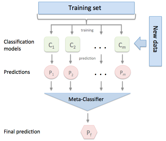
10.5.5 Stacking Ensemble Classic ML Models
# 5 fold stacking ensembling with 3 Repeated Stratified 10-Fold cross validation

# get a stacking ensemble of models
def get_stacking():
  # define the base models
  level0 = list()
  level0.append(('logreg', LogisticRegression()))
  level0.append(('knn', KNeighborsClassifier()))
  level0.append(('rforest', RandomForestClassifier()))
  level0.append(('etree', ExtraTreesClassifier()))
  level0.append(('svm', SVC()))

  # define meta learner model
  level1 = LogisticRegression()

  # define the stacking ensemble
  model = StackingClassifier(estimators=level0, final_estimator=level1, cv=5)
  return model

# get a list of models to evaluate
def get_models():
  models = dict()
  models['logreg'] = LogisticRegression()
  models['knn'] = KNeighborsClassifier()
  models['rforest'] = RandomForestClassifier()
  models['etree'] = ExtraTreesClassifier()
  models['svm'] = SVC()
  models['stacking'] = get_stacking()
  return models

# evaluate a give model using cross-validation
def evaluate_model(model, X, y):
	cv = RepeatedStratifiedKFold(n_splits=10, n_repeats=3, random_state=1)
	scores = cross_val_score(model, X, y, scoring='accuracy', cv=cv, n_jobs=-1, error_score='raise')
	return scores

# get the models to evaluate
models = get_models()

# evaluate the models and store results
results, names = list(), list()

printmd("**Model Evaluation :**")

for name, model in models.items():
	scores = evaluate_model(model, X, y)
	results.append(scores)
	names.append(name)
	print('>%s, cross-validation score - mean  : %.3f std: (%.3f)' % (name, np.mean(scores), np.std(scores)))

printmd("<br>")

# plot model performance for comparison
font_size = 15
plt.figure(figsize=(10,8))
plt.boxplot(results, labels=names, showmeans=True)

plt.title("Model Performance",  fontsize=font_size)
plt.xlabel("ML Models", fontsize=font_size)
plt.ylabel("Cross-val Score",  fontsize=font_size)
plt.xticks(fontsize=font_size)
plt.yticks(fontsize=font_size)

plt.show()


# credit : https://machinelearningmastery.com/stacking-ensemble-machine-learning-with-python

Classic ML models perform poorly in comparison with Gradient Boosting models
11 Conclusion
- Number of months the customer has stayed with the company (tenure) and the contract term of the customer (contract) are the most important features that have strong correlation with churn of the customer
- Results from statiscial hypotheses testing reflects similarity with model feature importance
- With 80/20 train/test split triple boosting stacking ensemble model achieved an AUC of ~0.85
12 Reference
- statstest
- parametric nonparametric tests healthknowledge - healthknowledge.org
- Feature Selection Method For Machine Learning - machinelearningmastery
- The Search for Categorical Correlation - towardsdatascience
- nonparametric statistical significance
- eta-squared - ResearchGate
- T-test examples - analyticsvidhya
- Nonparametric Statistical Hypothesis Tests - machinelearningmastery
- kendalls-tau
- Chi-Squared Test for Machine Learning
- parametric-and-non-parametric-data
- mann-whitney-u-test for non-parametric
- Point-biserial correlation, Phi, & Cramer's V
- Theia's Uncertainity
- non-parametric-correlation-for-continuous-and-dichotomous-variables
- Effect Size Wiki
- categorical correlation
- correlation_ratio dython
- 7. Tetrachoric’s correlation
- chi-square
- kruskal-wallis - statisticshowto
- Everything You Need To Know About Correlation