01 Molecular Geometry Analysis
The purpose of this project is to introduce you to fundamental Python programming techniques in the context of a scientific problem, viz. the calculation of the internal coordinates (bond lengths, bond angles, dihedral angles), moments of inertia, and rotational constants of a polyatomic molecule. A concise set of instructions for this project may be found here.
Original authors (Crawford, et al.) thank Dr. Yukio Yamaguchi of the University of Georgia for the original version of this project.
Solution of this project could be {download}solution_01.py.
# Following os.chdir code is only for thebe (live code), since only in thebe default directory is /home/jovyan
import os
if os.getcwd().split("/")[-1] != "Project_01":
    os.chdir("source/Project_01")
from solution_01 import Molecule as SolMol
Step 1: Read the Coordinate Data from Input
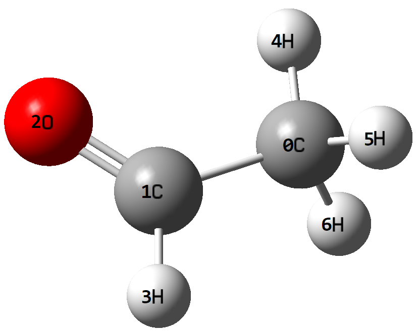
The input to the program is the set of Cartesian coordinates of the atoms (in bohr) and their associated atomic numbers. A sample molecule (acetaldehyde) to use as input to the program is:
7
6  0.000000000000     0.000000000000     0.000000000000
6  0.000000000000     0.000000000000     2.845112131228
8  1.899115961744     0.000000000000     4.139062527233
1 -1.894048308506     0.000000000000     3.747688672216
1  1.942500819960     0.000000000000    -0.701145981971
1 -1.007295466862    -1.669971842687    -0.705916966833
1 -1.007295466862     1.669971842687    -0.705916966833
The first line above is the number of atoms (an integer), while the remaining lines contain the z-values (atom charges) and x-, y-, and z-coordinates of each atom (one integer followed by three double-precision floating-point numbers). This input file({download}input/acetaldehyde.dat) along with a few other test cases can be found in this repository in the input directory.
After downloading the file to your computer (to a file called geom.dat, for example), you must open the file, read the data from each line into appropriate variables, and finally close the file.
{admonition}
:class: dropdown

In Python, using `open` and `close` can easily handle file I/Os:

```python
>>> f = open("input/acetaldehyde.dat", "r")
>>> # handle file `f`
>>> f.close()
```

However, there's more elegent way to do this by `with`:

```python
>>> with open("input/acetaldehyde.dat", "r") as f:
>>>     pass  # handle file `f`
```

The latter code is prefered. Using `with` would automatically close file, avoiding possibilities that programmer forget inserting a line to close file.
{admonition}
:class: dropdown

Handling multiple words (decimals, floats as strings) is relatively easy in Python. For example,

```python
>>> "6  0.000000000000     0.000000000000     0.000000000000".split()
['6', '0.000000000000', '0.000000000000', '0.000000000000']
```

However, these are string types. One need to transform to proper types to enable calculation afterwards.
{admonition}
:class: dropdown

There are two ways in python.

An intutive way to do this is generating a list to store z-values (as array), and list of list to store coordinates (as matrix). Notice do not use string type, for the sake of convenience of calculation tasks afterwards. It is also the most used way to store array/matrix in C++ and fortran90+. In FORTRAN77, one must use array to store matrix, along with it's leading dimension.

Another way is to use numpy. For example,

```python
>>> arr = np.array([
... ["0.0", "0.1"],
... ["2.5", "4.6"],
... ], dtype=float)
>>> arr
array([[0. , 0.1],
       [2.5, 4.6]])
```

Numpy can be extremely powerful, not only it wraps many array/matrix properties (raw data, dimension, type, etc.) into one class (`numpy.ndarray`), but also offers powerful operations in very concise way (matrix multiplication, SVD, tensor contraction, etc.).

Learning some essentials of NumPy can prove to be useful. In this document, NumPy will be the default array/matrix/tensor storage structure. Other robust array/matrix/tensor engines could be PyTorch/TensorFlow, etc.
{admonition}
:class: dropdown

What defines a molecule is somehow complicated. Not only it's atom charges, but also its coordinates. We can derive bond lengths, angles, etc. only from molecule information. We may term atom charges and coordinates as *Attribiutes*; they are variables and information describing molecule, like adjectives in gramma. We may term how we generate bond lengths, angles, etc. as *Methods*; they are functions, mapping from molecule information to some properties we desire, like verbs in gramma.

An example to construct molecule class may be

```python
class Molecule:

    def __init__(self):
        self.atom_charges = NotImplemented  # type: np.ndarray
        self.atom_coords = NotImplemented  # type: np.ndarray
        self.natm = NotImplemented  # type: int

    def construct_from_dat_file(self, file_path: str):
        # Input: Read file from `file_path`
        # Attribute modification: Obtain atom charges to `self.atom_charges`
        # Attribute modification: Obtain coordinates to `self.atom_coords`
        # Attribute modification: Obtain atom numbers in molecule to `self.natm`
        raise NotImplementedError("Reader need to fill this method function!")
```

For convenience, redundant variable `self.natm` (number of atoms in molecule) is also included as *Attribute*. It can be easily obtained by counting length of atom charges array `self.atom_charges`.
Implementation
If
moleis an instance ofMoleculeclass, and it's acetaldehyde molecule, thenmole.atom_chargesshould be a NumPy array with shape (7, )mole.atom_coordsshould be a NumPy array with shape (7, 3) (we use array instead of matrix, just convention; like any array/matrix in TensorFlow/PyTorch is termed tensor)mole.natmshould be an integer
Reader should fill all NotImplementedError in the following code (notice that NotImplemented is coded intentionally, not the same to NotImplementedError):
import numpy as np


class Molecule:

    def __init__(self):
        self.atom_charges = NotImplemented  # type: np.ndarray
        self.atom_coords = NotImplemented  # type: np.ndarray
        self.natm = NotImplemented  # type: int

    def construct_from_dat_file(self, file_path: str):
        # Input: Read file from `file_path`
        # Attribute modification: Obtain atom charges to `self.atom_charges`
        # Attribute modification: Obtain coordinates to `self.atom_coords`
        # Attribute modification: Obtain atom numbers in molecule to `self.natm`
        raise NotImplementedError("About 5~15 lines of code")
Solution
Following is reference output. Reader may repeat the output results with his/hers own implementation.
sol_mole = SolMol()
sol_mole.construct_from_dat_file("input/acetaldehyde.dat")
print(sol_mole.atom_charges)
print(sol_mole.atom_coords)
print(sol_mole.natm)
[6 6 8 1 1 1 1]
[[ 0.          0.          0.        ]
 [ 0.          0.          2.84511213]
 [ 1.89911596  0.          4.13906253]
 [-1.89404831  0.          3.74768867]
 [ 1.94250082  0.         -0.70114598]
 [-1.00729547 -1.66997184 -0.70591697]
 [-1.00729547  1.66997184 -0.70591697]]
7
Step 2: Bond Lengths
Calculate the interatomic distances using the expression:
$$ R_{ij} = \sqrt{(x_i - x_j)^2 + (y_i - y_j)^2 + (z_i - z_j)^2} $$where $x$, $y$, and $z$ are Cartesian coordinates and $i$ and $j$ denote atomic indices.
Print all bond lengths $R_{ij}$ in Bohr.
{admonition}
:class: dropdown

Before writing program, we need to ask ourselfs, that what information do we need to definitely define bond length. Actually, we need the two atoms ($i, j$ as subscripts of $R_{ij}$), and molecule coordinates ($x_i, y_i, z_i$). So we define the program as

```python
def bond_length(mole: Molecule, i: int, j: int) -> float:
    # Input: `i`, `j` index of molecule's atom
    # Output: Bond length from atom `i` to atom `j`
    raise NotImplementedError("Reader need to fill this method function!")
```
{admonition}
:class: dropdown

Directly programming by the expression of $R_{ij}$ is very intutive. However, this expression can also be written as

$$
R_{ij} = |\boldsymbol{r}_i - \boldsymbol{r}_j | := \Vert \boldsymbol{r}_i - \boldsymbol{r}_j \Vert_2
$$

where $\boldsymbol{r}_i = (x_i, y_i, z_i)$. $R_{ij}$ could be also termed as $L_2$ (Frobenius) norm of vector $\boldsymbol{r}_i - \boldsymbol{r}_j$, and $L_2$ norm of vector is implemented by NumPy (`numpy.linalg.norm`). See [NumPy API](https://numpy.org/doc/stable/reference/generated/numpy.linalg.norm.html) for its usage.

Using `numpy.linalg.norm` is preferred, but not compulsory at this stage.

If reader is not ready to use NumPy, python's standard library `math` is prefered to make sqrt calculation. For example, norm of vector $(0, 3, 4)$ could be calculated as

```python
>>> import math
>>> math.sqrt(0**2 + 3**2 + 4**2)
5.0
```
{admonition}
:class: dropdown

We may use python's default printing utilities for debugging:

```python
>>> print(0, 1, 2.845112131228)
0 1 2.845112131228
```

However, if we want to format printing string, we may use `str.format` method function. Reader may search `python string format` in search engines for more details. For example, if we want to print atom indexes in 3-char-long decimals and bond length in 10-char-long-5-after-decimal-point, we may write program as

```python
>>> print("{:3d} - {:3d}: {:10.5f} Bohr".format(0, 1, 2.845112131228))
  0 -   1:    2.84511 Bohr
```

You may wish to implement another function `print_bond_length` to realize this feature.
{admonition}
:class: dropdown

We need to print all bond length information in function `print_bond_length`, as Step 2 Hint 3 stated. Note that bond between atom 1 - atom 2 is the same to atom 2 - atom 1. So, reader should notice the range for each loop. In the following code, atom index `j` is always larger than `i`:

```python
for i in range(mole.natm):
    for j in range(i + 1, mole.natm):
        raise NotImplementedError  # Reader should complete printing code
```
{admonition}
:class: dropdown

We have discussed how to construct `Molecule` class in Step 1 Hint 4. However, we could regard `bond_length` function defined in Step 2 Hint 1 as method function of `Molecule` class. Though this is somehow not "pythonic", one can add method function (or attribute) after class construction, in fashion like C++. But we note that python is more flexable than C++ when handling methods in class, since in C++, although method implementation is not required when constructing class, one still need to declare signiture of function. In python, there's no need declaring function, so we just do implementations.

In this case, if we have defined function `bond_length` in Step 2 Hint 1, we just make the following statement to add this function to `Molecule` class:

```python
Molecule.bond_length = bond_length
```

We note that when calling `bond_length`, we need use

```python
bond_length(mole, i, j)
```

but when calling `Molecule.bond_length`, we need use

```python
mole.bond_length(i, j)
```

The first parameter `mole: Molecule` in `Molecule.bond_length`, like other (non-static) method functions, is equivalent to `self`.
Implementation
Reader should fill all NotImplementedError in the following code:
def bond_length(mole: Molecule, i: int, j: int) -> float:
    # Input: `i`, `j` index of molecule's atom
    # Output: Bond length from atom `i` to atom `j`
    raise NotImplementedError("About 1~3 lines of code")

Molecule.bond_length = bond_length
def print_bond_length(mole: Molecule):
    # Usage: Print all bond length
    print("=== Bond Length ===")
    for i in range(mole.natm):
        for j in range(i + 1, mole.natm):
            raise NotImplementedError("Exactly 1 line of code")

Molecule.print_bond_length = print_bond_length
Solution
sol_mole.print_bond_length()
=== Bond Length ===
  0 -   1:    2.84511 Bohr
  0 -   2:    4.55395 Bohr
  0 -   3:    4.19912 Bohr
  0 -   4:    2.06517 Bohr
  0 -   5:    2.07407 Bohr
  0 -   6:    2.07407 Bohr
  1 -   2:    2.29803 Bohr
  1 -   3:    2.09811 Bohr
  1 -   4:    4.04342 Bohr
  1 -   5:    4.05133 Bohr
  1 -   6:    4.05133 Bohr
  2 -   3:    3.81330 Bohr
  2 -   4:    4.84040 Bohr
  2 -   5:    5.89151 Bohr
  2 -   6:    5.89151 Bohr
  3 -   4:    5.87463 Bohr
  3 -   5:    4.83836 Bohr
  3 -   6:    4.83836 Bohr
  4 -   5:    3.38971 Bohr
  4 -   6:    3.38971 Bohr
  5 -   6:    3.33994 Bohr
Step 3: Bond Angles
Calculate bond angles. For example, the angle, $\phi_{ijk}$, between atoms $i$-$j$-$k$, where $j$ is the central atom is given by:
$$ \cos \phi_{ijk} = \boldsymbol{e}_{ji} \cdot \boldsymbol{e}_{jk} $$where the $\boldsymbol{e}_{ij}$ are unit vectors between the atoms, e.g.,
$$ e_{ij}^x = - \frac{x_i - x_j}{R_{ij}}, \quad e_{ij}^y = - \frac{y_i - y_j}{R_{ij}}, \quad e_{ij}^z = - \frac{z_i - z_j}{R_{ij}} $$Print all valid bond angles $\phi_{ijk}$ (with bond length $R_{ij} < 3 \, \mathsf{Bohr}$ and $R_{jk} < 3 \, \mathsf{Bohr}$, and $\phi_{ijk} > 90^\circ$) in degree.
Original C++ project suggests storing unit vectors in memory. However, this python project will generate unit vectors on-the-fly. Also, the final result of this step is a little different to the original project.
{admonition}
:class: dropdown

From the definition above, we may state that

$$
\boldsymbol{e}_{ij} = \frac{\boldsymbol{r}_j - \boldsymbol{r}_i}{| \boldsymbol{r}_j - \boldsymbol{r}_i |}
$$

It is a combined opeation of vector substraction, $L_2$ norm, and vector divided by numerical value. In NumPy, they are quite easy to achieve.
{admonition}
:class: dropdown

We used inner product between $\boldsymbol{e}_{ji}$ and $\boldsymbol{e}_{jk}$ in the fomular above:

$$
\cos \phi_{ijk} = \boldsymbol{e}_{ji} \cdot \boldsymbol{e}_{jk} = e_{ji}^x e_{jk}^x + e_{ji}^y e_{jk}^y + e_{ji}^z e_{jk}^z
$$

In NumPy, there are multiple ways to achieve vector inner product. An intutive way is using `numpy.inner` (see [NumPy API](https://numpy.org/doc/stable/reference/generated/numpy.inner.html)). For example,

```python
>>> np.inner([-1, 1, 2], [3, 9, 5])
16
```

Other ways could be `numpy.dot`, `numpy.tensordot`, `numpy.einsum`, `np.multiply` with `np.sum`.
{admonition}
:class: dropdown

We need calculate arccos value of vector inner product. In NumPy, `numpy.arccos` can do this job. Without NumPy, there's still `math.acos`.

Note that we need to print angle in degree, so we need to multiply result by $180 / \pi$.
{admonition}
:class: dropdown

From the description, we should know that bond angle 1-2-3 is the same to 3-2-1. However, we regard 1-2-3 as different bond angle to 2-1-3. If bond length of 1-2 is larger than 4 Angstrom, then we silent all bond angles 1-2-\*; but if bond length of 1-3 is larger than 3 Angstrom, as well as 1-2, 2-3 shorter than 3 Angstrom, we still print bond angle 1-2-3.

Utilizing that the sum of interior angles of a triangle is 180°, we know that for any three atoms, they have utmost one angle larger than 90°.
Implementation
Reader should fill all NotImplementedError in the following code:
def bond_unit_vector(mole: Molecule, i: int, j: int) -> np.ndarray:
    # Input: `i`, `j` index of molecule's atom
    # Output: Unit vector of bond from atom `i` to atom `j`
    raise NotImplementedError("About 1~5 lines of code")

Molecule.bond_unit_vector = bond_unit_vector
def bond_angle(mole: Molecule, i: int, j: int, k: int) -> float:
    # Input: `i`, `j`, `k` index of molecule's atom; where `j` is the central atom
    # Output: Bond angle for atoms `i`-`j`-`k`
    raise NotImplementedError("About 3~5 lines of code")

Molecule.bond_angle = bond_angle
def is_valid_angle(mole: Molecule, i: int, j: int, k: int) -> bool:
    # Input: `i`, `j`, `k` index of molecule's atom; where `j` is the central atom
    # Output: Test if `i`-`j`-`k` is a valid bond angle
    #         if i != j != k
    #         and if i-j and j-k bond length smaller than 3 Angstrom,
    #         and if angle i-j-k > 90 degree
    raise NotImplementedError("About 1~5 lines of code")

Molecule.is_valid_angle = is_valid_angle
def print_bond_angle(mole: Molecule):
    # Usage: Print all bond angle i-j-k which is considered as valid angle
    raise NotImplementedError("About 5~20 lines of code")

Molecule.print_bond_angle = print_bond_angle
Solution
For this solution, there could be different outputs, such as angle 0-1-2 should be equal to 2-1-0. Such kind of minor differences could be tolerated. However, angle values, number of valid angles, etc. should be exactly the same.
sol_mole.print_bond_angle()
=== Bond Angle ===
  0 -   1 -   2:  124.26831 Degree
  0 -   1 -   3:  115.47934 Degree
  1 -   0 -   4:  109.84706 Degree
  1 -   0 -   5:  109.89841 Degree
  1 -   0 -   6:  109.89841 Degree
  4 -   0 -   5:  109.95368 Degree
  4 -   0 -   6:  109.95368 Degree
  5 -   0 -   6:  107.25265 Degree
  2 -   1 -   3:  120.25235 Degree
Step 4: Out-of-Plane Angles
Calculate out-of-plane angles. For example, the angle $\theta_{ijkl}$ for atom $i$ out of the plane containing atoms $j$-$k$-$l$ (with $k$ as the central atom, connected to $i$) is given by:
$$ \sin \theta_{ijkl} = \frac{\boldsymbol{e}_{kj} \times \boldsymbol{e}_{kl}}{\sin \phi_{jkl}} \cdot \boldsymbol{e}_{ki} $$Print all valid out-of-plane angles (bond angle $\phi_{jkl}$ should be valid bond angle, and bond length $R_{ki} < 3 \, \mathsf{Bohr}$) in degree. Note that situation of $\sin \phi_{jkl} = 0$ could occasionally (especially Molecule HCN or H2C=C=CH2), so excluding this kind of situation is encouraged.
{admonition}
:class: dropdown

Cross product of two arrays (length of array is 3) $\boldsymbol{c} = \boldsymbol{a} \times \boldsymbol{b}$ is defined as

$$
\begin{align}
c_x &= a_y b_z - a_z b_y \\
c_y &= a_z b_x - a_x b_z \\
c_z &= a_x b_y - a_y b_x
\end{align}
$$

In NumPy, `numpy.cross` ([NumPy API](https://numpy.org/doc/stable/reference/generated/numpy.cross.html)) could fulfill this feature.

```python
>>> np.cross([5, 2, 3], [7, 8, 9])
array([ -6, -24,  26])
```
{admonition}
:class: dropdown

Actually, when implementing arcsin operation, one may encounter `RuntimeWarning` from NumPy:

```python
>>> np.arcsin(-1.000000000000001)
<stdin>:1: RuntimeWarning: invalid value encountered in arcsin
nan
```

To avoid such kind of error, one need to make sure the value passed into `numpy.arcsin` is not larger than 1 nor smaller than -1, strictly. One may also assert that the passed value is not too large or too small, in case of internal programming mistakes.

```python
>>> theta = -1.000000000000001
>>> assert(np.abs(theta) < 1 + 1e-7)  # make sure that theta is not too wrong, in case of programming mistakes
>>> theta = np.sign(theta) if np.abs(theta) > 1 else theta  # make theta bounded between -1 to 1
>>> np.arcsin(theta)
-1.5707963267948966
```
Implementation
Reader should fill all NotImplementedError in the following code:
def out_of_plane_angle(mole: Molecule, i: int, j: int, k: int, l: int) -> float:
    # Input: `i`, `j`, `k`, `l` index of molecule's atom; where `k` is the central atom, and angle is i - j-k-l
    # Output: Out-of-plane bond angle for atoms `i`-`j`-`k`-`l`
    raise NotImplementedError("About 3~8 lines of code")

Molecule.out_of_plane_angle = out_of_plane_angle
def is_valid_out_of_plane_angle(mole: Molecule, i: int, j: int, k: int, l: int) -> bool:
    # Input: `i`, `j`, `k`, `l` index of molecule's atom; where `k` is the central atom, and angle is i - j-k-l
    # Output: Test if `i`-`j`-`k` is a valid out-of-plane bond angle
    #         if i != j != k != l
    #         and if angle j-k-l is valid bond angle
    #         and if i-k bond length smaller than 3 Angstrom
    #         and bond angle of j-k-l is not linear
    raise NotImplementedError("About 1~5 lines of code")

Molecule.is_valid_out_of_plane_angle = is_valid_out_of_plane_angle
def print_out_of_plane_angle(mole: Molecule):
    # Usage: Print all out-of-plane bond angle i-j-k-l which is considered as valid
    raise NotImplementedError("About 6~15 lines of code")

Molecule.print_out_of_plane_angle = print_out_of_plane_angle
Solution
Difference of output may also be tolerated in this solution.
sol_mole.print_out_of_plane_angle()
=== Out-of-Plane Angle ===
  3 -   0 -   1 -   2:    0.00000 Degree
  2 -   0 -   1 -   3:    0.00000 Degree
  5 -   1 -   0 -   4:  -53.62632 Degree
  6 -   1 -   0 -   4:   53.62632 Degree
  4 -   1 -   0 -   5:   53.65153 Degree
  6 -   1 -   0 -   5:  -56.27711 Degree
  4 -   1 -   0 -   6:  -53.65153 Degree
  5 -   1 -   0 -   6:   56.27711 Degree
  1 -   4 -   0 -   5:  -53.67878 Degree
  6 -   4 -   0 -   5:   56.19462 Degree
  1 -   4 -   0 -   6:   53.67878 Degree
  5 -   4 -   0 -   6:  -56.19462 Degree
  1 -   5 -   0 -   6:  -54.97706 Degree
  4 -   5 -   0 -   6:   54.86999 Degree
  0 -   2 -   1 -   3:    0.00000 Degree
Step 5: Torsion/Dihedral Angles
Calculate torsional angles. For example, the torsional angle $\tau_{ijkl}$ for the atom connectivity $i$-$j$-$k$-$l$ is given by:
$$ \cos \tau_{ijkl} = \frac{(\boldsymbol{e}_{ji} \times \boldsymbol{e}_{jk}) \cdot (\boldsymbol{e}_{kj} \times \boldsymbol{e}_{kl})}{\sin \phi_{ijk} \cdot \sin \phi_{jkl}} $$Print all valid dihedral angles ($i, j, k$ and $j, k, l$ constructs a valid angle, where $j, k$ should be bonded or $R_{jk} < 3 \, \mathsf{Bohr}$) in degree.
Implementation
Reader should fill all NotImplementedError in the following code:
def dihedral_angle(mole: Molecule, i: int, j: int, k: int, l: int) -> float:
    # Input: `i`, `j`, `k`, `l` index of molecule's atom; where `k` is the central atom, and angle is i - j-k-l
    # Output: Dihedral angle for atoms `i`-`j`-`k`-`l`
    raise NotImplementedError("About 3~8 lines of code")

Molecule.dihedral_angle = dihedral_angle
def is_valid_dihedral_angle(mole: Molecule, i: int, j: int, k: int, l: int) -> bool:
    # Input: `i`, `j`, `k`, `l` index of molecule's atom; where `k` is the central atom, and angle is i - j-k-l
    # Output: Test if `i`-`j`-`k` is a valid dihedral bond angle
    #         if i != j != k != l
    #         and if i, j, k construct a valid bond angle (with j-k bonded)
    #         and if j, k, l construct a valid bond angle (with j-k bonded)
    raise NotImplementedError("About 1~5 lines of code")

Molecule.is_valid_dihedral_angle = is_valid_dihedral_angle
def print_dihedral_angle(mole: Molecule):
    # Usage: Print all dihedral bond angle i-j-k-l which is considered as valid
    raise NotImplementedError("About 6~15 lines of code")

Molecule.print_dihedral_angle = print_dihedral_angle
Solution
Difference of output may also be tolerated in this solution.
sol_mole.print_dihedral_angle()
=== Dihedral Angle ===
  2 -   0 -   1 -   3:  180.00000 Degree
  2 -   0 -   1 -   4:    0.00000 Degree
  2 -   0 -   1 -   5:  121.09759 Degree
  2 -   0 -   1 -   6:  121.09759 Degree
  3 -   0 -   1 -   4:  180.00000 Degree
  3 -   0 -   1 -   5:   58.90241 Degree
  3 -   0 -   1 -   6:   58.90241 Degree
  4 -   0 -   1 -   5:  121.09759 Degree
  4 -   0 -   1 -   6:  121.09759 Degree
  5 -   0 -   1 -   6:  117.80483 Degree
  1 -   0 -   4 -   5:  121.06434 Degree
  1 -   0 -   4 -   6:  121.06434 Degree
  5 -   0 -   4 -   6:  117.87131 Degree
  1 -   0 -   5 -   4:  121.03351 Degree
  1 -   0 -   5 -   6:  119.43447 Degree
  4 -   0 -   5 -   6:  119.53201 Degree
  1 -   0 -   6 -   4:  121.03351 Degree
  1 -   0 -   6 -   5:  119.43447 Degree
  4 -   0 -   6 -   5:  119.53201 Degree
  0 -   1 -   2 -   3:  180.00000 Degree
  0 -   1 -   3 -   2:  180.00000 Degree
Step 6: Center-of-Mass Translation
Find the center of mass of the molecule:
$$ \boldsymbol{r}_\mathrm{c.m.} = \left. \sum_{i} m_i \boldsymbol{r}_i \right/ \sum_{i} m_i $$or in its components
$$ x_\mathrm{c.m.} = \left. \sum_i m_i x_i \right/ \sum_i m_i , \quad y_\mathrm{c.m.} = \left. \sum_i m_i y_i \right/ \sum_i m_i , \quad z_\mathrm{c.m.} = \left. \sum_i m_i z_i \right/ \sum_i m_i $$where $m_i$ is the mass of atom $i$ and the summation runs over all atoms in the molecule.
Translate the input coordinates of the molecule to the center-of-mass.
We use isotopic-averaged atom mass, so the final results may be different to the original Crawford's project at $10^{-3} \, \mathsf{a.u.}$ level.
{admonition}
:class: dropdown

An excellent source for atomic masses and other physical constants is the [National Institute of Standard and Technology (NIST) website](https://physics.nist.gov/cgi-bin/Compositions/stand_alone.pl).

For python users, one may find package [molmass](https://github.com/cgohlke/molmass) useful.
Implementation
def center_of_mass(mole: Molecule) -> np.ndarray or list:
    # Output: Center of mass for this molecule
    raise NotImplementedError("About 5~10 lines of code")

Molecule.center_of_mass = center_of_mass
Solution
sol_mole.center_of_mass()
array([0.64475065, 0. , 2.31636762])
Step 7: Principal Moments of Inertia
Calculate elements of the moment of inertia tensor.
Diagonal:
$$ I_{xx} = \sum_i m_i (\tilde y_i^2 + \tilde z_i^2), \quad I_{yy} = \sum_i m_i (\tilde z_i^2 + \tilde x_i^2) \, \quad I_{zz} = \sum_i m_i (\tilde x_i^2 + \tilde y_i^2) $$Off-diagonal (add a negative sign):
$$ I_{xy} = I_{yx} = - \sum_i m_i \tilde x_i \tilde y_i, \quad I_{yz} = I_{zy} = - \sum_i m_i \tilde y_i \tilde z_i, \quad I_{zx} = I_{xz} = - \sum_i m_i \tilde z_i \tilde x_i $$Calculate eigenvalue of inertia tensor to obtain the principal moments of inertia:
$$ I_a \leqslant I_b \leqslant I_c $$Report the moments of inertia in $\mathsf{amu \cdot Bohr^2}$, $\mathsf{amu \cdot {\buildrel_{\circ} \over{\mathsf{A}}}{}^2}$, $\mathsf{g \cdot cm^2}$.
Note that $\tilde x_i, \tilde y_i, \tilde z_i$ in the equations above are translated by center of mass:
$$ \tilde x_i = x_i - x_\mathrm{c.m.}, \quad \tilde y_i = y_i - y_\mathrm{c.m.}, \quad \tilde z_i = z_i - z_\mathrm{c.m.} $$Based on the relative values of the principal moments, determine the molecular rotor type. Criterion of equality and far larger/smaller could be set to $10^{-4} \mathsf{amu \cdot Bohr^2}$.
Spherical: $I_a = I_b = I_c$
Linear: $I_a \ll I_b = I_c$
Prolate: $I_a < I_b = I_c$
Oblate: $I_a = I_b < I_c$
Asymmetric: $I_a \neq I_b \neq I_c$
{admonition}
:class: dropdown

Eigenvalue $\lambda$ of moments of inertia matrix can be obtained as

$$
\left\vert
\begin{matrix}
I_{xx} - \lambda & I_{xy} & I_{xz} \\
I_{yx} & I_{yy} - \lambda & I_{yz} \\
I_{zx} & I_{zy} & I_{zz} - \lambda
\end{matrix}
\right\vert = 0
$$

This leads to a cubic equation in $\lambda$, which one can solve directly.

However, solving symmetric matrix by program is usually called *diagonalization*. This can be done by `numpy.linalg.eigh` which returns eigenvalues and eigenvectors ([NumPy API](https://numpy.org/doc/stable/reference/generated/numpy.linalg.eigh.html)) or `numpy.linalg.eigvalsh` which only returns eigenvalues ([NumPy API](https://numpy.org/doc/stable/reference/generated/numpy.linalg.eigvalsh.html)).
{admonition}
:class: dropdown

Lots of useful and precise physical constants are available at the [National Institute of Standards and Technology website](https://physics.nist.gov/cuu/Constants/index.html?/codata86.html).

For python, `scipy.constants` ([SciPy API](https://docs.scipy.org/doc/scipy/reference/constants.html)) offers lots of constants and unit conversion utilities.
Implementation
Reader should fill all NotImplementedError in the following code:
def moment_of_inertia(mole: Molecule) -> np.ndarray or list:
    # Output: Principle of moments of intertia
    raise NotImplementedError("About 4~25 lines of code")

Molecule.moment_of_inertia = moment_of_inertia
def print_moment_of_interia(mole: Molecule):
    # Output: Print moments of inertia in amu bohr2, amu Å2, and g cm2
    raise NotImplementedError("About 3~15 lines of code")

Molecule.print_moment_of_interia = print_moment_of_interia
def type_of_moment_of_interia(mole: Molecule) -> str:
    # Output: Judge which type of moment of interia is
    raise NotImplementedError("About 7~11 lines of code")

Molecule.type_of_moment_of_interia = type_of_moment_of_interia
Solution
Value of principles of moment of interia:
sol_mole.print_moment_of_interia()
In      amu bohr^2:   3.19751875e+01   1.78736281e+02   1.99467661e+02
In  amu angstrom^2:   8.95396445e+00   5.00512562e+01   5.58566339e+01
In          g cm^2:   1.48684078e-39   8.31120663e-39   9.27521227e-39
Type of interia:
sol_mole.type_of_moment_of_interia()
'Asymmetric'
Step 8: Rotational Constants
Compute the rotational constants in $\mathsf{cm}^{-1}$ and $\mathsf{MHz}$:
$$ A = \frac{h}{8 \pi^2 c I_a} , \quad B = \frac{h}{8 \pi^2 c I_b} , \quad C = \frac{h}{8 \pi^2 c I_c} $$where $A \geqslant B \geqslant C$.
Implementation
Reader should fill all NotImplementedError in the following code:
def rotational_constants(mole: Molecule) -> np.ndarray or list:
    # Output: Rotational constant in cm^-1
    raise NotImplementedError("About 1~10 lines of code")

Molecule.rotational_constants = rotational_constants
Solution
Compute the rotational constants in $\mathsf{cm}^{-1}$
sol_mole.rotational_constants()
array([1.88270004, 0.33680731, 0.30180174])
Test Cases
Acetaldehyde
- Input file: {download}
input/acetaldehyde.dat
sol_mole = SolMol()
sol_mole.construct_from_dat_file("input/acetaldehyde.dat")
sol_mole.print_solution_01()
=== Atom Charges ===
[6 6 8 1 1 1 1]
=== Coordinates ===
[[ 0.          0.          0.        ]
 [ 0.          0.          2.84511213]
 [ 1.89911596  0.          4.13906253]
 [-1.89404831  0.          3.74768867]
 [ 1.94250082  0.         -0.70114598]
 [-1.00729547 -1.66997184 -0.70591697]
 [-1.00729547  1.66997184 -0.70591697]]
=== Bond Length ===
  0 -   1:    2.84511 Bohr
  0 -   2:    4.55395 Bohr
  0 -   3:    4.19912 Bohr
  0 -   4:    2.06517 Bohr
  0 -   5:    2.07407 Bohr
  0 -   6:    2.07407 Bohr
  1 -   2:    2.29803 Bohr
  1 -   3:    2.09811 Bohr
  1 -   4:    4.04342 Bohr
  1 -   5:    4.05133 Bohr
  1 -   6:    4.05133 Bohr
  2 -   3:    3.81330 Bohr
  2 -   4:    4.84040 Bohr
  2 -   5:    5.89151 Bohr
  2 -   6:    5.89151 Bohr
  3 -   4:    5.87463 Bohr
  3 -   5:    4.83836 Bohr
  3 -   6:    4.83836 Bohr
  4 -   5:    3.38971 Bohr
  4 -   6:    3.38971 Bohr
  5 -   6:    3.33994 Bohr
=== Bond Angle ===
  0 -   1 -   2:  124.26831 Degree
  0 -   1 -   3:  115.47934 Degree
  1 -   0 -   4:  109.84706 Degree
  1 -   0 -   5:  109.89841 Degree
  1 -   0 -   6:  109.89841 Degree
  4 -   0 -   5:  109.95368 Degree
  4 -   0 -   6:  109.95368 Degree
  5 -   0 -   6:  107.25265 Degree
  2 -   1 -   3:  120.25235 Degree
=== Out-of-Plane Angle ===
  3 -   0 -   1 -   2:    0.00000 Degree
  2 -   0 -   1 -   3:    0.00000 Degree
  5 -   1 -   0 -   4:  -53.62632 Degree
  6 -   1 -   0 -   4:   53.62632 Degree
  4 -   1 -   0 -   5:   53.65153 Degree
  6 -   1 -   0 -   5:  -56.27711 Degree
  4 -   1 -   0 -   6:  -53.65153 Degree
  5 -   1 -   0 -   6:   56.27711 Degree
  1 -   4 -   0 -   5:  -53.67878 Degree
  6 -   4 -   0 -   5:   56.19462 Degree
  1 -   4 -   0 -   6:   53.67878 Degree
  5 -   4 -   0 -   6:  -56.19462 Degree
  1 -   5 -   0 -   6:  -54.97706 Degree
  4 -   5 -   0 -   6:   54.86999 Degree
  0 -   2 -   1 -   3:    0.00000 Degree
=== Dihedral Angle ===
  2 -   0 -   1 -   3:  180.00000 Degree
  2 -   0 -   1 -   4:    0.00000 Degree
  2 -   0 -   1 -   5:  121.09759 Degree
  2 -   0 -   1 -   6:  121.09759 Degree
  3 -   0 -   1 -   4:  180.00000 Degree
  3 -   0 -   1 -   5:   58.90241 Degree
  3 -   0 -   1 -   6:   58.90241 Degree
  4 -   0 -   1 -   5:  121.09759 Degree
  4 -   0 -   1 -   6:  121.09759 Degree
  5 -   0 -   1 -   6:  117.80483 Degree
  1 -   0 -   4 -   5:  121.06434 Degree
  1 -   0 -   4 -   6:  121.06434 Degree
  5 -   0 -   4 -   6:  117.87131 Degree
  1 -   0 -   5 -   4:  121.03351 Degree
  1 -   0 -   5 -   6:  119.43447 Degree
  4 -   0 -   5 -   6:  119.53201 Degree
  1 -   0 -   6 -   4:  121.03351 Degree
  1 -   0 -   6 -   5:  119.43447 Degree
  4 -   0 -   6 -   5:  119.53201 Degree
  0 -   1 -   2 -   3:  180.00000 Degree
  0 -   1 -   3 -   2:  180.00000 Degree
=== Center of Mass ===
   0.64475    0.00000    2.31637
=== Moments of Inertia ===
In      amu bohr^2:   3.19751875e+01   1.78736281e+02   1.99467661e+02
In  amu angstrom^2:   8.95396445e+00   5.00512562e+01   5.58566339e+01
In          g cm^2:   1.48684078e-39   8.31120663e-39   9.27521227e-39
Type:  Asymmetric
=== Rotational Constants ===
In cm^-1:      1.88270      0.33681      0.30180
In   MHz:  56441.92712  10097.22927   9047.78849
Allene
- Input file: {download}
input/allene.dat
sol_mole = SolMol()
sol_mole.construct_from_dat_file("input/allene.dat")
sol_mole.print_solution_01()
=== Atom Charges ===
[6 6 6 1 1 1 1]
=== Coordinates ===
[[ 0.          0.          1.88972599]
 [ 2.55113008  0.          1.88972599]
 [-2.55113008  0.          1.88972599]
 [ 3.49599308  1.15721611  0.73250988]
 [ 3.49599308 -1.15721611  3.0469421 ]
 [-3.49599308 -1.15721611  0.73250988]
 [-3.49599308  1.15721611  3.0469421 ]]
=== Bond Length ===
  0 -   1:    2.55113 Bohr
  0 -   2:    2.55113 Bohr
  0 -   3:    3.86009 Bohr
  0 -   4:    3.86009 Bohr
  0 -   5:    3.86009 Bohr
  0 -   6:    3.86009 Bohr
  1 -   2:    5.10226 Bohr
  1 -   3:    1.88973 Bohr
  1 -   4:    1.88973 Bohr
  1 -   5:    6.26466 Bohr
  1 -   6:    6.26466 Bohr
  2 -   3:    6.26466 Bohr
  2 -   4:    6.26466 Bohr
  2 -   5:    1.88973 Bohr
  2 -   6:    1.88973 Bohr
  3 -   4:    3.27310 Bohr
  3 -   5:    7.36508 Bohr
  3 -   6:    7.36508 Bohr
  4 -   5:    7.36508 Bohr
  4 -   6:    7.36508 Bohr
  5 -   6:    3.27310 Bohr
=== Bond Angle ===
  1 -   0 -   2:  180.00000 Degree
  0 -   1 -   3:  120.00000 Degree
  0 -   1 -   4:  120.00000 Degree
  0 -   2 -   5:  120.00000 Degree
  0 -   2 -   6:  120.00000 Degree
  3 -   1 -   4:  120.00000 Degree
  5 -   2 -   6:  120.00000 Degree
=== Out-of-Plane Angle ===
  4 -   0 -   1 -   3:    0.00000 Degree
  3 -   0 -   1 -   4:    0.00000 Degree
  6 -   0 -   2 -   5:    0.00000 Degree
  5 -   0 -   2 -   6:    0.00000 Degree
  0 -   3 -   1 -   4:    0.00000 Degree
  0 -   5 -   2 -   6:    0.00000 Degree
=== Dihedral Angle ===
  2 -   0 -   1 -   3:   90.00000 Degree
  2 -   0 -   1 -   4:   90.00000 Degree
  3 -   0 -   1 -   4:  180.00000 Degree
  1 -   0 -   2 -   5:   90.00000 Degree
  1 -   0 -   2 -   6:   90.00000 Degree
  5 -   0 -   2 -   6:  180.00000 Degree
  0 -   1 -   3 -   4:  180.00000 Degree
  0 -   1 -   4 -   3:  180.00000 Degree
  0 -   2 -   5 -   6:  180.00000 Degree
  0 -   2 -   6 -   5:  180.00000 Degree
=== Center of Mass ===
   0.00000    0.00000    1.88973
=== Moments of Inertia ===
In      amu bohr^2:   1.07982664e+01   2.11013373e+02   2.11013373e+02
In  amu angstrom^2:   3.02382256e+00   5.90897626e+01   5.90897626e+01
In          g cm^2:   5.02117550e-40   9.81208592e-39   9.81208592e-39
Type:  Prolate
=== Rotational Constants ===
In cm^-1:      5.57494      0.28529      0.28529
In   MHz: 167132.49483   8552.73379   8552.73379
Benzene
- Input file: {download}
input/benzene.dat
sol_mole = SolMol()
sol_mole.construct_from_dat_file("input/benzene.dat")
sol_mole.print_solution_01()
=== Atom Charges ===
[6 6 6 6 6 6 1 1 1 1 1 1]
=== Coordinates ===
[[ 0.00000000e+00  0.00000000e+00  0.00000000e+00]
 [ 0.00000000e+00  0.00000000e+00  2.61644846e+00]
 [ 2.26591048e+00  0.00000000e+00  3.92467249e+00]
 [ 4.53182108e+00  0.00000000e+00  2.61644839e+00]
 [ 4.53182108e+00  0.00000000e+00 -1.32281000e-07]
 [ 2.26591069e+00  0.00000000e+00 -1.30822415e+00]
 [ 2.26591069e+00 -0.00000000e+00 -3.33421820e+00]
 [ 6.28638327e+00  0.00000000e+00 -1.01299708e+00]
 [ 6.28638324e+00  0.00000000e+00  3.62944532e+00]
 [ 2.26591048e+00  0.00000000e+00  5.95066654e+00]
 [-1.75456219e+00  0.00000000e+00  3.62944541e+00]
 [-1.75456216e+00 -0.00000000e+00 -1.01299693e+00]]
=== Bond Length ===
  0 -   1:    2.61645 Bohr
  0 -   2:    4.53182 Bohr
  0 -   3:    5.23290 Bohr
  0 -   4:    4.53182 Bohr
  0 -   5:    2.61645 Bohr
  0 -   6:    4.03130 Bohr
  0 -   7:    6.36748 Bohr
  0 -   8:    7.25889 Bohr
  0 -   9:    6.36748 Bohr
  0 -  10:    4.03130 Bohr
  0 -  11:    2.02599 Bohr
  1 -   2:    2.61645 Bohr
  1 -   3:    4.53182 Bohr
  1 -   4:    5.23290 Bohr
  1 -   5:    4.53182 Bohr
  1 -   6:    6.36748 Bohr
  1 -   7:    7.25889 Bohr
  1 -   8:    6.36748 Bohr
  1 -   9:    4.03130 Bohr
  1 -  10:    2.02599 Bohr
  1 -  11:    4.03130 Bohr
  2 -   3:    2.61645 Bohr
  2 -   4:    4.53182 Bohr
  2 -   5:    5.23290 Bohr
  2 -   6:    7.25889 Bohr
  2 -   7:    6.36748 Bohr
  2 -   8:    4.03130 Bohr
  2 -   9:    2.02599 Bohr
  2 -  10:    4.03130 Bohr
  2 -  11:    6.36748 Bohr
  3 -   4:    2.61645 Bohr
  3 -   5:    4.53182 Bohr
  3 -   6:    6.36748 Bohr
  3 -   7:    4.03130 Bohr
  3 -   8:    2.02599 Bohr
  3 -   9:    4.03130 Bohr
  3 -  10:    6.36748 Bohr
  3 -  11:    7.25889 Bohr
  4 -   5:    2.61645 Bohr
  4 -   6:    4.03130 Bohr
  4 -   7:    2.02599 Bohr
  4 -   8:    4.03130 Bohr
  4 -   9:    6.36748 Bohr
  4 -  10:    7.25889 Bohr
  4 -  11:    6.36748 Bohr
  5 -   6:    2.02599 Bohr
  5 -   7:    4.03130 Bohr
  5 -   8:    6.36748 Bohr
  5 -   9:    7.25889 Bohr
  5 -  10:    6.36748 Bohr
  5 -  11:    4.03130 Bohr
  6 -   7:    4.64244 Bohr
  6 -   8:    8.04095 Bohr
  6 -   9:    9.28488 Bohr
  6 -  10:    8.04095 Bohr
  6 -  11:    4.64244 Bohr
  7 -   8:    4.64244 Bohr
  7 -   9:    8.04095 Bohr
  7 -  10:    9.28488 Bohr
  7 -  11:    8.04095 Bohr
  8 -   9:    4.64244 Bohr
  8 -  10:    8.04095 Bohr
  8 -  11:    9.28488 Bohr
  9 -  10:    4.64244 Bohr
  9 -  11:    8.04095 Bohr
 10 -  11:    4.64244 Bohr
=== Bond Angle ===
  0 -   1 -   2:  120.00000 Degree
  1 -   0 -   5:  120.00000 Degree
  0 -   1 -  10:  120.00000 Degree
  1 -   0 -  11:  120.00000 Degree
  0 -   5 -   4:  120.00000 Degree
  0 -   5 -   6:  120.00000 Degree
  5 -   0 -  11:  120.00000 Degree
  1 -   2 -   3:  120.00000 Degree
  1 -   2 -   9:  120.00000 Degree
  2 -   1 -  10:  120.00000 Degree
  2 -   3 -   4:  120.00000 Degree
  2 -   3 -   8:  120.00000 Degree
  3 -   2 -   9:  120.00000 Degree
  3 -   4 -   5:  120.00000 Degree
  3 -   4 -   7:  120.00000 Degree
  4 -   3 -   8:  120.00000 Degree
  4 -   5 -   6:  120.00000 Degree
  5 -   4 -   7:  120.00000 Degree
=== Out-of-Plane Angle ===
 10 -   0 -   1 -   2:    0.00000 Degree
 11 -   1 -   0 -   5:    0.00000 Degree
  2 -   0 -   1 -  10:    0.00000 Degree
  5 -   1 -   0 -  11:    0.00000 Degree
  6 -   0 -   5 -   4:    0.00000 Degree
  4 -   0 -   5 -   6:    0.00000 Degree
  1 -   5 -   0 -  11:    0.00000 Degree
  9 -   1 -   2 -   3:    0.00000 Degree
  3 -   1 -   2 -   9:    0.00000 Degree
  0 -   2 -   1 -  10:    0.00000 Degree
  8 -   2 -   3 -   4:    0.00000 Degree
  4 -   2 -   3 -   8:    0.00000 Degree
  1 -   3 -   2 -   9:    0.00000 Degree
  7 -   3 -   4 -   5:    0.00000 Degree
  5 -   3 -   4 -   7:    0.00000 Degree
  2 -   4 -   3 -   8:    0.00000 Degree
  0 -   4 -   5 -   6:    0.00000 Degree
  3 -   5 -   4 -   7:    0.00000 Degree
=== Dihedral Angle ===
  2 -   0 -   1 -   5:    0.00000 Degree
  2 -   0 -   1 -  10:  180.00000 Degree
  2 -   0 -   1 -  11:  180.00000 Degree
  5 -   0 -   1 -  10:  180.00000 Degree
  5 -   0 -   1 -  11:  180.00000 Degree
 10 -   0 -   1 -  11:    0.00000 Degree
  1 -   0 -   5 -   4:    0.00000 Degree
  1 -   0 -   5 -   6:  180.00000 Degree
  1 -   0 -   5 -  11:  180.00000 Degree
  4 -   0 -   5 -   6:  180.00000 Degree
  4 -   0 -   5 -  11:  180.00000 Degree
  6 -   0 -   5 -  11:    0.00000 Degree
  1 -   0 -  11 -   5:  180.00000 Degree
  0 -   1 -   2 -   3:    0.00000 Degree
  0 -   1 -   2 -   9:  180.00000 Degree
  0 -   1 -   2 -  10:  180.00000 Degree
  3 -   1 -   2 -   9:  180.00000 Degree
  3 -   1 -   2 -  10:  180.00000 Degree
  9 -   1 -   2 -  10:    0.00000 Degree
  0 -   1 -  10 -   2:  180.00000 Degree
  1 -   2 -   3 -   4:    0.00000 Degree
  1 -   2 -   3 -   8:  180.00000 Degree
  1 -   2 -   3 -   9:  180.00000 Degree
  4 -   2 -   3 -   8:  180.00000 Degree
  4 -   2 -   3 -   9:  180.00000 Degree
  8 -   2 -   3 -   9:    0.00000 Degree
  1 -   2 -   9 -   3:  180.00000 Degree
  2 -   3 -   4 -   5:    0.00000 Degree
  2 -   3 -   4 -   7:  180.00000 Degree
  2 -   3 -   4 -   8:  180.00000 Degree
  5 -   3 -   4 -   7:  180.00000 Degree
  5 -   3 -   4 -   8:  180.00000 Degree
  7 -   3 -   4 -   8:    0.00000 Degree
  2 -   3 -   8 -   4:  180.00000 Degree
  0 -   4 -   5 -   3:    0.00000 Degree
  0 -   4 -   5 -   6:  180.00000 Degree
  0 -   4 -   5 -   7:  180.00000 Degree
  3 -   4 -   5 -   6:  180.00000 Degree
  3 -   4 -   5 -   7:  180.00000 Degree
  6 -   4 -   5 -   7:    0.00000 Degree
  3 -   4 -   7 -   5:  180.00000 Degree
  0 -   5 -   6 -   4:  180.00000 Degree
=== Center of Mass ===
   2.26591    0.00000    1.30822
=== Moments of Inertia ===
In      amu bohr^2:   3.11839639e+02   3.11839704e+02   6.23679344e+02
In  amu angstrom^2:   8.73239929e+01   8.73240110e+01   1.74648004e+02
In          g cm^2:   1.45004902e-38   1.45004932e-38   2.90009833e-38
Type:  Oblate
=== Rotational Constants ===
In cm^-1:      0.19305      0.19305      0.09652
In   MHz:   5787.40152   5787.40032   2893.70046
References
Wilson, E. B.; Decius, J. C.; Cross, P. C. Molecular Vibrations Dover Publication Inc., 1980.
ISBN-13: 978-0486639413