Building a Production ML Pipeline For Gravitational Wave Detection

Alec Gunny$^{*,1}$, Ethan Marx$^1$, William Benoit$^2$, Deep Chatterjee$^1$, Michael Coughlin$^2$, Katya Govorkova$^1$, Philip Harris$^1$, Erik Katsavounidis$^1$, Eric Moreno$^1$, Rafia Omer$^2$, Ryan Raikman$^1$, Muhammed Saleem$^2$

_{^{1 - Massachussetts Institute of Technology}}

_{^{2 - University of Minnesota}}

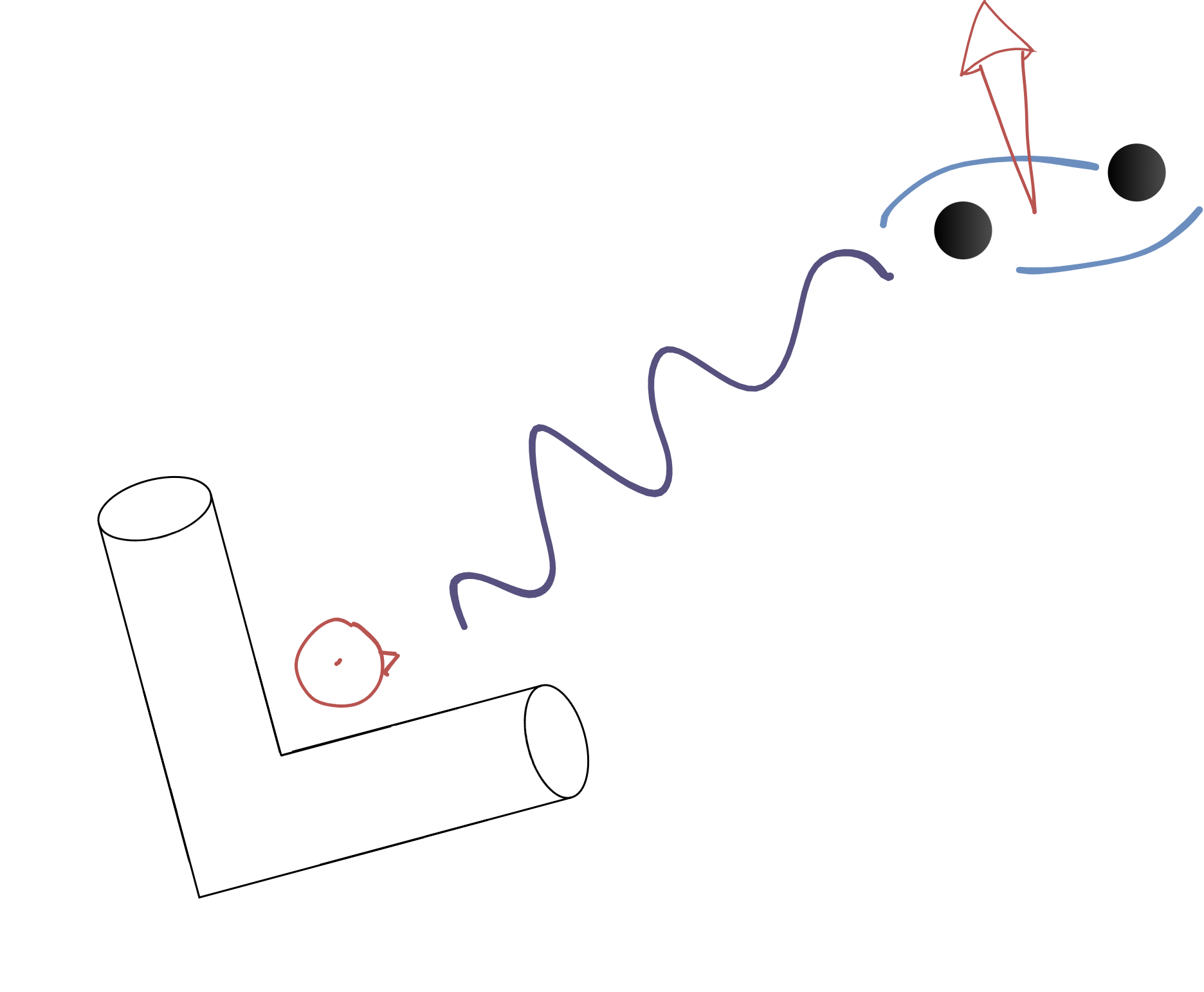
Gravitational Waves

Large-scale astrophysical events ripple fabric of spacetime, detected via earth-based interferometers Low-latency detection of events allows for localization and follow-up ML algorithms - small inference compute Binary blackhole mergers are an "easy" problem to prove capabilities and build infra

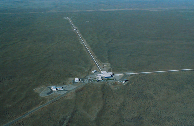
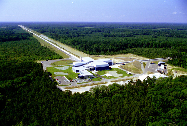
Focusing here on LIGO inteferometers Hanford, Washington Livingston, Louisiana

https://www.ligo.caltech.edu

ML in practice

• Writing ML training code is easy: model.fit(X, y)
• Doing good science with ML is hard
  • Largest gains from development of domain specific ecosystems
  • Fast tools with intuitive APIs that map on to familiar concepts
• GW physics has a great software ecosystem
  • Robust simulations, good priors, etc., but none optimized for ML
• Introduce here two libraries to seed such an ecosystem

ml4gw - PyTorch training utilitieshermes - Inference-as-a-Service deployment utilities

ML4GW

• GitHub organization containing libraries, projects, etc.
• Always room for more collaborators!

https://github.com/ML4GW

Some implementation notes

• Not live, but run in one fell swoop (try it!)
• NOT about
  • How to train an ML model
  • torch or lightning or gwpy or pycbc or bokeh
  • Even really ml4gw or hermes
• IS about demonstrating how domain-optimized tools can deliver more robust models and systems
  • Hide or skim details where necessary to stay focused
• "What about..." Great question! Good tools let us answer good questions with more confidence
• Full paper on BBH detection coming, stay posted

Some implementation notes

Coding in slides makes you space conscious, so I'll get some imports and constant definitions out of the way here.

import h5py
import numpy as np
from utils import plotting

ifos = ["H1", "L1"]
sample_rate = 2048

Loading BokehJS ...

3 minute crash course in gravitational wave data processing

! ls data

background.hdf5  signals.hdf5

background.hdf5

Real, open data observed by the Hanford (H1) and Livingston (L1) interferometers between April 1st and April 22nd 2019

• 1 week for training/validation, 2 weeks for test

with h5py.File("data/background.hdf5", "r") as f:
    for split in ["train", "valid", "test"]:
        num_segments = len(f[split])
        duration = sum([len(v[ifos[0]]) / sample_rate for v in f[split].values()])
        print(
            "{} segments in {} split, corresponding to {:0.2f} h of livetime".format(
                num_segments, split, duration / 3600
            )
        )

8 segments in train split, corresponding to 38.82 h of livetime
3 segments in valid split, corresponding to 18.64 h of livetime
22 segments in test split, corresponding to 111.96 h of livetime

background.hdf5

What's this data look like?

with h5py.File("data/background.hdf5", "r") as f:
    dataset = f["train"]["1238175433-17136"]  # start timestamp of segment-duration
    background = {i: dataset[i][:sample_rate * 10] for i in ifos} # plot first 10s
t = np.arange(sample_rate * 10) / sample_rate
plotting.plot_timeseries(t, **background)

signals.hdf5

Simulated waveforms generated by gravitational wave events along with the parameters of those events

• Train and validation datasets contain raw waveform polarizations

with h5py.File("data/signals.hdf5") as f:
    for split in ["train", "valid"]:
        dataset = f[split]["polarizations"]["cross"]
        num_signals, size = dataset.shape
        print("{} {} s signals in {} split".format(len(dataset), size/sample_rate, split))

50000 4.0 s signals in train split
10000 4.0 s signals in valid split

signals.hdf5

And what do these signals look like?

with h5py.File("data/signals.hdf5") as f:
    # let's look at a loud training signal
    split = f["train"]
    idx = split["parameters"]["snr"][:].argmax()
    signal = {i: split["polarizations"][i][idx] for i in ["cross", "plus"]}
t = np.arange(size) / sample_rate
plotting.plot_timeseries(t, **signal)

• Inteferometers act as antennae that respond linearly to polarizations
• Function of relative locations/orientations of detectors and source

from pycbc.detector import Detector

sky_params = ["declination", "right_ascension", "polarization"]
with h5py.File("data/signals.hdf5", "r") as f:
    params = {i: f[f"train/parameters/{i}"][idx] for i in sky_params}

responses = {}
for ifo in ifos:
    detector = Detector(ifo)
    fp, fc = detector.antenna_pattern(t_gps=1238175433, **params)
    response = ht = fp * signal["plus"] + fc * signal["cross"]  # call observed strain h(t)
    responses[ifo] = ht
plotting.plot_timeseries(t, **responses)

• Projection from polarization $\rightarrow$ response introduces
  • phase shifts due to differences in arrival times
  • differences in relative amplitudes due to slight differences in polarization
• Test signals have been pre-projected so that we can analyze it as if it was a real event
• All signals have been rejection sampled to ensure their signal-to-noise ratio (SNR) is $\geq$ 4

Back to detection

What examples can we give a neural network that will help it learn to detect presence of signal?

• "Loudest" part of signal is in last 0.5-1 seconds, near the coalescence
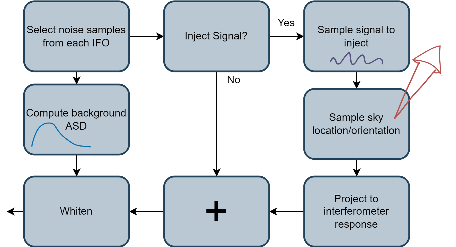
• Signals add simply to background noise, i.e. $h(t) = n(t) + s(t)$
• So why don't we:
  • Take short windows of background, say 1s
  • Add simulated/projected signals to ~50% of them
  • Train a binary classification network on this data

What would this data look like? What does the network "see"?

injected, uninjected = {}, {}
for ifo in ifos:
    # I'm actually going to grab 2 seconds for reasons that will become clear momentarily
    bg = background[ifo][-2 * sample_rate:]
    uninjected[ifo] = bg
    injected[ifo] = bg.copy()
    injected[ifo][:sample_rate] += responses[ifo][-sample_rate:]
t = np.arange(len(bg)) / sample_rate
plotting.plot_side_by_side(uninjected, injected, t, titles=["Before injection", "After injection"])

No major difference - but this shouldn't be suprising: background strain is $\mathcal{O}(10^{-19})$, waveforms are $\mathcal{O}(10^{-22})$

Well we tried

Thank you!

• Most of background is low frequency content - 10-30Hz
• Most of signal is in 60-500Hz
• Emphasize signal by whitening the data: normalize frequency content by amplitude spectral density (ASD) of background

from gwpy.timeseries import TimeSeries

asd_length, fftlength = 8, 2
asds = {}
for ifo in ifos:
    bg = TimeSeries(background[ifo], sample_rate=sample_rate)
    asds[ifo] = bg.crop(0, asd_length).asd(fftlength, method="median")
plotting.plot_spectral(**asds)

for ifo in ifos:
    for src in [injected, uninjected]:
        x = TimeSeries(src[ifo], sample_rate=sample_rate)
        x = x.whiten(asd=asds[ifo], fduration=1)  # fduration is response time of filter
        x = x.crop(0.5, 1.5)  # edges are corrupted by filter settle-in
        src[ifo] = x.value
t = t[sample_rate // 2: -sample_rate // 2]
plotting.plot_side_by_side(uninjected, injected, t, titles=["Before injection", "After injection"])

So a quick review of how we'll generate the samples on which to train our neural network:

Training the network

How do we do this in practice?

• Too much background to fit in memory at once
• Not sure if we can do it in real-time
• Start by generating fixed train and validation datasets up front, then fit on these

• make_dataset will take care of these steps using the traditional GW software stack
• Don't need to worry about the details, but clock the throughput

from utils.data import make_dataset

background_f = h5py.File("data/background.hdf5")
signal_f = h5py.File("data/signals.hdf5")
with background_f, signal_f:
    datasets = {}
    for split in ["train", "valid"]:
        datasets[split] = make_dataset(
            ifos,
            background_f[split],
            signal_f[split],
            kernel_length=1,
            fduration=1,
            psd_length=8,
            fftlength=2,
            sample_rate=sample_rate,
            highpass=32
        )

100%|██████████████████████████████████████████████████████████████████████████████████████| 100000/100000 [1:02:17<00:00, 26.76it/s]
100%|██████████████████████████████████████████████████████████████████████████████████████████| 20000/20000 [12:16<00:00, 27.14it/s]

What does our data look like now?

for split in ["train", "valid"]:
    X, y = datasets[split]
    num_signal = (y == 1).sum()
    num_background = (y == 0).sum()
    print("{} samples of shape {} in {} split, {} signal and {} background".format(
        len(X), X.shape[1:], split, num_signal, num_background
    ))

100000 samples of shape (2, 2048) in train split, 50000 signal and 50000 background
20000 samples of shape (2, 2048) in valid split, 10000 signal and 10000 background

Start by defining a simple lightning model that will train a 1D ResNet architecture on our dataset.

Details not really important

import torch
from lightning import pytorch as pl
from torchmetrics.classification import BinaryAUROC
from utils.nn import ResNet

class VanillaDetectionModel(pl.LightningModule):
    def __init__(
        self,
        learning_rate: float = 0.001,
        batch_size: int = 1024,
        max_fpr: float = 1e-2  # only measure ourselves on FPRs close to where we'll operate
    ) -> None:
        super().__init__()
        self.save_hyperparameters()
        self.nn = ResNet(len(ifos), layers=[2, 3, 4, 2])
        self.metric = BinaryAUROC(max_fpr=max_fpr)

    def forward(self, X):
        return self.nn(X)

    def training_step(self, batch):
        X, y = batch
        y_hat = self(X)
        loss = torch.nn.functional.binary_cross_entropy_with_logits(y_hat, y)
        self.log("train_loss", loss, on_step=True, prog_bar=True)
        return loss

    def validation_step(self, batch):
        X, y = batch
        y_hat = self(X)
        self.metric.update(y_hat, y)
        self.log("valid_auroc", self.metric, on_epoch=True, prog_bar=True)

    def configure_optimizers(self):
        parameters = self.nn.parameters()
        optimizer = torch.optim.AdamW(parameters, self.hparams.learning_rate)
        scheduler = torch.optim.lr_scheduler.OneCycleLR(
            optimizer,
            self.hparams.learning_rate,
            pct_start=0.1,
            total_steps=self.trainer.estimated_stepping_batches
        )
        scheduler_config = dict(scheduler=scheduler, interval="step")
        return dict(optimizer=optimizer, lr_scheduler=scheduler_config)

    def configure_callbacks(self):
        chkpt = pl.callbacks.ModelCheckpoint(monitor="valid_auroc", mode="max")
        return [chkpt]

    def make_dataset(self, split):
        X, y = datasets[split]
        X, y = torch.Tensor(X), torch.Tensor(y)
        return torch.utils.data.TensorDataset(X, y)

    def train_dataloader(self):
        dataset = self.make_dataset("train")
        return torch.utils.data.DataLoader(
            dataset,
            batch_size=self.hparams.batch_size,
            shuffle=True,
            pin_memory=True
        )

    def val_dataloader(self):
        dataset = self.make_dataset("valid")
        return torch.utils.data.DataLoader(
            dataset,
            batch_size=self.hparams.batch_size * 4,
            shuffle=False,
            pin_memory=True
        )

Now let's fit the model to our pre-generated dataset

model = VanillaDetectionModel(batch_size=1024, learning_rate=0.02)
trainer = pl.Trainer(
    max_epochs=20,
    precision="16-mixed",
    log_every_n_steps=5,
    logger=pl.loggers.CSVLogger("logs", name="vanilla-expt"),
    callbacks=[pl.callbacks.RichProgressBar()]
)
trainer.fit(model)

Missing logger folder: logs/vanilla-expt

┏━━━┳━━━━━━━━┳━━━━━━━━━━━━━┳━━━━━━━━┓
┃   ┃ Name   ┃ Type        ┃ Params ┃
┡━━━╇━━━━━━━━╇━━━━━━━━━━━━━╇━━━━━━━━┩
│ 0 │ nn     │ ResNet      │  4.7 M │
│ 1 │ metric │ BinaryAUROC │      0 │
└───┴────────┴─────────────┴────────┘

Trainable params: 4.7 M                                                                                            
Non-trainable params: 0                                                                                            
Total params: 4.7 M                                                                                                
Total estimated model params size (MB): 18                                                                         

Loss curve shows clear signs of overfitting

plotting.plot_run("vanilla-expt")

Keep the best model weights for inference later

best_vanilla_weights = trainer.checkpoint_callback.best_model_path

Mission accomplished?

• So it looks like we perform... well? Who knows, we'll address inference/evaluation later
• Consider all the ways we threw out data/priors/physics to make this work
  • Didn't use even close to all our background
  • Even worse when you consider we can shift IFOs wrt one another
  • Only got to observe waveforms from one sky location/distance
  • Only got to observe waveforms inserted in one particular noise background
• We could just generate a larger dataset, but just kicks the can

What if we did this in real time during training?

• Take advantage of our data and physics to build more robust models
  • Our data generation throughput was ~40 samples/s
  • Our NN throughput was ~3500 samples/s
  • Even if we get a lot faster, existing tools insufficient for real-time use

Enter ml4gw

Library of torch utilities for common GW tasks/transforms

• Align with existing APIs
• pip installable
• GPU accelerated, tensor-ized operations ensure efficient utilization
• Auto-differentiation means we can take gradients through ops - build physics into models

import ml4gw

Enter ml4gw

Let's re-implement our sample-generation code using ml4gw dataloaders and transforms

Start by clearing out the GPU:

import gc

def flush():
    gc.collect()
    torch.cuda.empty_cache()
    torch.cuda.reset_peak_memory_stats()

flush()

Training with ml4gw

Start by defining a new model that will generate samples in real time.

from ml4gw import distributions, gw, transforms
from ml4gw.dataloading import ChunkedTimeSeriesDataset, Hdf5TimeSeriesDataset
from ml4gw.utils.slicing import sample_kernels

class Ml4gwDetectionModel(VanillaDetectionModel):
    """
    Model with additional methods for performing our
    preprocessing augmentations in real-time on the GPU.
    Also loads training background in chunks from disk,
    then samples batches from chunks.

    Note that the training and validation steps themselves
    don't need to change at all: all we're doing is building
    better ways of getting data to _feed_ to the training
    step.
    """

    def __init__(
        self,
        ifos: list[str],
        kernel_length: float,
        fduration: float,
        psd_length: float,
        sample_rate: float,
        fftlength: float,
        chunk_length: float = 128,  # we'll talk about chunks in a second
        reads_per_chunk: int = 40,
        highpass: float = 32,
        **kwargs
    ) -> None:
        super().__init__(**kwargs)

        # real-time transformations defined at torch Modules
        self.spectral_density = transforms.SpectralDensity(
            sample_rate, fftlength, average="median", fast=True
        )
        self.whitener = transforms.Whiten(fduration, sample_rate, highpass=highpass)

        # get some geometry information about
        # the interferometers we're going to project to
        detector_tensors, vertices = gw.get_ifo_geometry(*ifos)
        self.register_buffer("detector_tensors", detector_tensors)
        self.register_buffer("detector_vertices", vertices)

        # define some sky parameter distributions
        self.declination = distributions.Cosine()
        self.polarization = distributions.Uniform(0, torch.pi)
        self.phi = distributions.Uniform(-torch.pi, torch.pi)  # relative RAs of detector and source

        # rather than sample distances, we'll sample target SNRs.
        # This way we can ensure we train our network on
        # signals that are actually detectable. We'll use a distribution
        # that looks roughly like our sampled SNR distribution
        self.snr = distributions.PowerLaw(4, 100, 3)

        # up front let's define some properties in units of samples
        self.kernel_size = int(kernel_length * sample_rate)
        self.window_size = self.kernel_size + int(fduration * sample_rate)
        self.psd_size = int(psd_length * sample_rate)

    def setup(self, stage):
        # lightning automatically calls this method before training starts.
        # We'll use it to load in all our signals up front, though we could
        # in principle sample these from disk for larger datasets
        with h5py.File("data/signals.hdf5", "r") as f:
            group = f["train"]["polarizations"]
            self.Hp = torch.Tensor(group["plus"][:])
            self.Hc = torch.Tensor(group["cross"][:])

    def sample_waveforms(self, batch_size: int) -> tuple[torch.Tensor, ...]:
        rvs = torch.rand(size=(batch_size,))
        mask = rvs > 0.5
        num_injections = mask.sum().item()

        idx = torch.randint(len(self.Hp), size=(num_injections,))
        hp = self.Hp[idx]
        hc = self.Hc[idx]
        return hc, hp, mask

    def project_waveforms(self, hc: torch.Tensor, hp: torch.Tensor) -> torch.Tensor:
        # sample sky parameters
        N = len(hc)
        declination = self.declination(N).to(hc)
        polarization = self.polarization(N).to(hc)
        phi = self.phi(N).to(hc)

        # project to interferometer response
        return gw.compute_observed_strain(
            declination,
            polarization,
            phi,
            detector_tensors=self.detector_tensors,
            detector_vertices=self.detector_vertices,
            sample_rate=self.hparams.sample_rate,
            cross=hc,
            plus=hp
        )

    def rescale_snrs(self, responses: torch.Tensor, psd: torch.Tensor) -> torch.Tensor:
        # make sure everything has the same number of frequency bins
        num_freqs = int(responses.size(-1) // 2) + 1
        if psd.size(-1) != num_freqs:
            psd = torch.nn.functional.interpolate(psd, size=(num_freqs,), mode="linear")
        snrs = gw.compute_network_snr(
            responses.double(), psd, self.hparams.sample_rate, self.hparams.highpass
        )

        N = len(responses)
        target_snrs = self.snr(N).to(snrs.device)
        weights = target_snrs / snrs
        return responses * weights.view(-1, 1, 1)

    def sample_kernels(self, responses: torch.Tensor) -> torch.Tensor:
        # slice off random views of each waveformto inject in arbitrary positions
        responses = responses[:, :, -self.window_size:]

        # pad so that at least half the kernel always contains signals
        pad = [0, int(self.window_size // 2)]
        responses = torch.nn.functional.pad(responses, pad)
        return sample_kernels(responses, self.window_size, coincident=True)

    @torch.no_grad()
    def augment(self, X: torch.Tensor) -> tuple[torch.Tensor, torch.Tensor]:
        # break off "background" from target kernel and compute its PSD
        # (in double precision since our scale is so small)
        background, X = torch.split(X, [self.psd_size, self.window_size], dim=-1)
        psd = self.spectral_density(background.double())

        # sample at most batch_size signals from our bank and move them to our
        # current device. Keep a mask that indicates which rows to inject in
        batch_size = X.size(0)
        hc, hp, mask = self.sample_waveforms(batch_size)
        hc, hp, mask = hc.to(X), hp.to(X), mask.to(X.device)

        # sample sky parameters and project to responses, then
        # rescale the response according to a randomly sampled SNR
        responses = self.project_waveforms(hc, hp)
        responses = self.rescale_snrs(responses, psd[mask])

        # randomly slice out a window of the waveform, add it
        # to our background, then whiten everything
        responses = self.sample_kernels(responses)
        X[mask] += responses.float()
        X = self.whitener(X, psd)

        # create labels, marking 1s where we injected
        y = torch.zeros((batch_size, 1), device=X.device)
        y[mask] = 1
        return X, y

    def on_after_batch_transfer(self, batch, _):
        # this is a parent method that lightning calls
        # between when the batch gets moved to GPU and
        # when it gets passed to the training_step.
        # Apply our augmentations here
        if self.trainer.training:
            batch = self.augment(batch)
        return batch

    def train_dataloader(self):
        # set up our dataloader so that the network "sees"
        # twice as many samples as the number of waveforms
        # during each epoch, so that on average it's going
        # through the training waveforms once in each epoch
        # (we sample with replacement, so it's not perfect).
        samples_per_epoch = 2 * len(self.Hp)
        batches_per_epoch = int((samples_per_epoch - 1) // self.hparams.batch_size) + 1
        batches_per_chunk = int(batches_per_epoch // 10)
        chunks_per_epoch = int(batches_per_epoch // batches_per_chunk) + 1

        # Hdf5TimeSeries dataset samples batches from disk.
        # In this instance, we'll make our batches really large so that
        # we can treat them as chunks to sample training batches from
        dataset = Hdf5TimeSeriesDataset(
            "data/background.hdf5",
            channels=self.hparams.ifos,
            kernel_size=int(self.hparams.chunk_length * self.hparams.sample_rate),
            batch_size=self.hparams.reads_per_chunk,
            batches_per_epoch=chunks_per_epoch,
            coincident=False,
            path="train"
        )

        # multiprocess this so there's always a new chunk ready when we need it
        dataloader = torch.utils.data.DataLoader(
            dataset,
            num_workers=2,
            pin_memory=True,
            persistent_workers=True
        )

        # sample batches to pass to our NN from the chunks loaded from disk
        return ChunkedTimeSeriesDataset(
            dataloader,
            kernel_size=self.window_size + self.psd_size,
            batch_size=self.hparams.batch_size,
            batches_per_chunk=batches_per_chunk,
            coincident=False
        )

Now instantiate the model with all our preprocessing parameters from before.

For dataloading, each chunk will read 20 random 128 second segments from our data on disk, from which we'll sample ~10% of batches in epoch.

model = Ml4gwDetectionModel(
    ifos,
    kernel_length=1,
    fduration=1,
    psd_length=8,
    sample_rate=sample_rate,
    fftlength=2,
    chunk_length=128,
    reads_per_chunk=20,
    highpass=32,
    learning_rate=0.005,
    batch_size=1024
)

Now let's fit this model, and see if we can do any better

logger = pl.loggers.CSVLogger("logs", name="ml4gw-expt")
trainer = pl.Trainer(
    max_epochs=20,
    precision="16-mixed",
    log_every_n_steps=5,
    logger=logger,
    callbacks=[pl.callbacks.RichProgressBar()]
)
trainer.fit(model)

Missing logger folder: logs/ml4gw-expt

┏━━━┳━━━━━━━━━━━━━━━━━━┳━━━━━━━━━━━━━━━━━┳━━━━━━━━┓
┃   ┃ Name             ┃ Type            ┃ Params ┃
┡━━━╇━━━━━━━━━━━━━━━━━━╇━━━━━━━━━━━━━━━━━╇━━━━━━━━┩
│ 0 │ nn               │ ResNet          │  4.7 M │
│ 1 │ metric           │ BinaryAUROC     │      0 │
│ 2 │ spectral_density │ SpectralDensity │      0 │
│ 3 │ whitener         │ Whiten          │      0 │
└───┴──────────────────┴─────────────────┴────────┘

Trainable params: 4.7 M                                                                                            
Non-trainable params: 0                                                                                            
Total params: 4.7 M                                                                                                
Total estimated model params size (MB): 18                                                                         

Much more robust loss curves, looks like still headroom to grow

plotting.plot_run("ml4gw-expt")

Save our best weights again

best_ml4gw_weights = trainer.checkpoint_callback.best_model_path

Inference and Evaluation

• So we've gone through the effort to train not just one but two models
• Validation scores are nice, but to deploy them we'll need meaningful metrics on a lot of data
• Key questions:
  • At a given NN output threshold, how many events per unit time do I expect to detect?
  • At the same threshold, how many false alarms per unit time do I expect to raise?
• Measure sensitive volume vs. false alarm rate using 2 weeks of time-shifted real background data
  • Mostly care about tail false alarm events, so quality of estimate heavily reliant on volume of data
  • In principle would want at least $\mathcal{O}$(years)
• For full details, see e.g. Tiwari 2017: https://arxiv.org/abs/1712.00482

Streaming inference

• High-frequency inference means NN inputs will contain redundant data
• Adopt a stateful streaming strategy to minimize I/O at the expense of introducing serial processing
• ml4gw contains some useful common stateful steps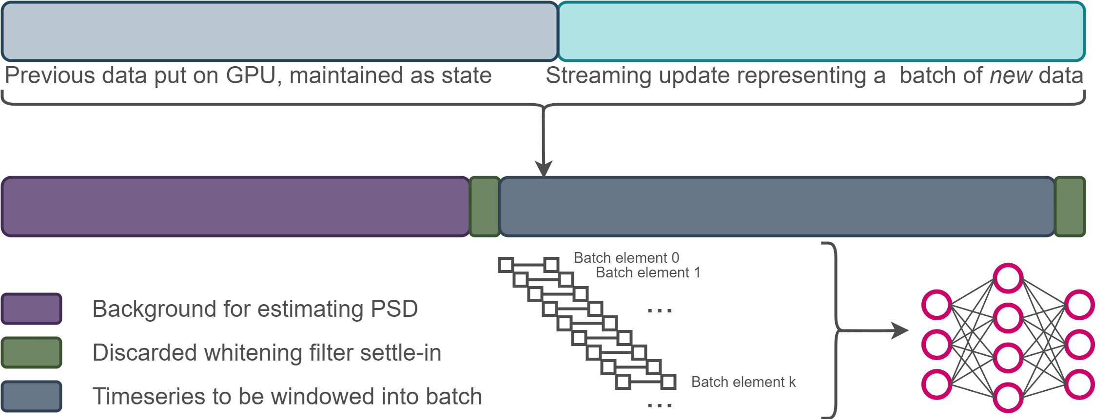

Local inference

• We'll start with the simplest approach: use our model and ml4gw preprocessing steps locally, in-memory
• Build a local stateful model we can use. See code for details

from utils import infer

batcher = infer.BatchGenerator(
    model.spectral_density,
    model.whitener,
    len(ifos),
    kernel_length=1,
    fduration=1,
    psd_length=64,
    inference_sampling_rate=8,
    sample_rate=sample_rate
)

Won't go into details of how we turn NN predictions into GW "events", see upcoming paper. Just need to define a function for generating that timeseries of NN predictions locally

class LocalInferenceFn:
    def __init__(self, model, chkpt_path, device="cuda") -> None:
        # load in our model checkpoint and set the nn
        # weights to the appropriate values
        checkpoint = torch.load(chkpt_path)
        state_dict = checkpoint["state_dict"]
        state_dict = {k.strip("n."): v for k, v in state_dict.items() if k.startswith("nn.")}
        model.nn.load_state_dict(state_dict)
        model.eval()
        self.model = model.to(device)
        self.device = device

    def __call__(self, streaming_iterator, pbar):
        bg_preds, fg_preds = [], []
        state = batcher.get_initial_state().to(self.device)
        for X in streaming_iterator:
            # move data onto GPU. X contains alternating
            # background and signal examples
            X = torch.Tensor(X).to(self.device)

            # now fan it out into a batch of overlapping samples
            # and retrieve the updated state
            batch, state = batcher(X, state)

            # do inference and separate out background and signal
            preds = self.model(batch)[:, 0]
            bg_preds.append(preds[::2])
            fg_preds.append(preds[1::2])

            # support a progress bar to keep track of everything
            pbar.update(1)

        # concatenate all our predictions into a timeseries of
        # NN outputs through which we'll comb for events
        bg_preds = torch.cat(bg_preds).cpu().numpy()
        fg_preds = torch.cat(fg_preds).cpu().numpy()
        return bg_preds, fg_preds

Now let's run inference for both our models and see

1. How long it takes
2. How they compare

infer_params = dict(
    ifos=ifos,
    kernel_length=1,  # length of input windows to network
    psd_length=64,  # how long of a segment to use for PSD estimation
    fduration=1,  # filter settle-in length
    inference_sampling_rate=8,  # how frequently to sample input windows
    batch_size=4096,
    pool_length=8  # how we keep from double counting events
)

vanilla_inference_fn = LocalInferenceFn(model, best_vanilla_weights)
vanilla_results = infer.infer(vanilla_inference_fn, **infer_params)

ml4gw_inference_fn = LocalInferenceFn(model, best_ml4gw_weights)
ml4gw_results = infer.infer(ml4gw_inference_fn, **infer_params)

100%|████████████████████████████████████████████████████████████████████████████████████████████| 3104/3104 [52:44<00:00,  1.02s/it]
100%|████████████████████████████████████████████████████████████████████████████████████████████| 3104/3104 [52:50<00:00,  1.02s/it]

How do these two models stack up against one another?

plotting.plot_evaluation(vanilla=vanilla_results, ml4gw=ml4gw_results)

Good to see the model trained with better physics perform better!

• But it took nearly an hour to analyze 2 weeks worth of data
• Need to scale up analyze useful lengths of time

Inference-as-a-Service

lightning has good distribution APIs, but some other things to consider

• Integration with other models in other frameworks (e.g. TensorFlow)
• Use of accelerated frameworks like TensorRT
• One model insufficient to saturate GPU compute - use multiple concurrent execution instances
• One data stream insufficient to saturate GPU compute - need multiple streams per GPU

Inference-as-a-Service

Central application responsible for executing model inference

• Accepts requests via lightweight client APIs
  • Abstracts implementation and framework details
• Asynchronously chedules requests from different clients
• Intra-device parallel execution ensures accelerators are saturated

Inference-as-a-Service - Triton Inference Server

NVIDIA's Triton Inference Server gets good performance out-of-the-box

• Stateful support can be tricky to navigate
• Configurations built around non-Pythonic protobufs
• No integration with frameworks to export/convert between formats easily
• Lots of boilerplate - most info should be built into model
  • Data types, shapes, tensor names, etc.
  • Recently added more support for inferring properties, but still lots of use cases where need to touch config

Enter hermes

Set of utilities for simplifying streaming inference-as-a-service deployment

• Not currently pip installable, but undergoing overhaul
• Keep an eye on repo for release in coming week

Let's

1. Export our preprocessor and NN using hermes
2. serve up this ensemble using Triton on 2 GPUs
3. See how much better our throughput gets

from hermes.quiver import ModelRepository, Platform

# create a fresh model repository and add a new entry for our nn to it.
# We'll export the model to an accelerated TensorRT executable in FP16.
# Note that our batch size is double: one for background and one for signals
repo = ModelRepository("repo", clean=True)
nn = repo.add("detector", platform=Platform.TENSORRT)
export_path = nn.export_version(
    model.nn.to("cpu"),
    input_shapes={"strain": (2 * infer_params["batch_size"], 2, sample_rate)},
    output_names=["detection_statistic"],
    use_fp16=True
)

[11/08/2023-00:40:05] [TRT] [W] TensorRT encountered issues when converting weights between types and that could affect accuracy.
[11/08/2023-00:40:05] [TRT] [W] If this is not the desired behavior, please modify the weights or retrain with regularization to adjust the magnitude of the weights.
[11/08/2023-00:40:05] [TRT] [W] Check verbose logs for the list of affected weights.
[11/08/2023-00:40:05] [TRT] [W] - 25 weights are affected by this issue: Detected subnormal FP16 values.
[11/08/2023-00:40:05] [TRT] [W] - 3 weights are affected by this issue: Detected values less than smallest positive FP16 subnormal value and converted them to the FP16 minimum subnormalized value.

So what's in our model repository now?

! ls repo

detector

! ls repo/detector

1  config.pbtxt

! ls repo/detector/1

model.plan

For our preprocessor, we'll need to use some utils to export it as a stateful model

from hermes.quiver.streaming.utils import add_streaming_model

update_size = batcher.step_size * infer_params["batch_size"]
preprocessor = add_streaming_model(
    repo,
    streaming_layer=batcher.to("cpu"),
    name="preprocessor",
    input_shape=(2, len(ifos), update_size),
    state_shapes=[(2, len(ifos), batcher.state_size)],
    platform=Platform.TORCHSCRIPT
)

/opt/demo/ml4gw/ml4gw/spectral.py:38: TracerWarning: Converting a tensor to a Python boolean might cause the trace to be incorrect. We can't record the data flow of Python values, so this value will be treated as a constant in the future. This means that the trace might not generalize to other inputs!
  if x.shape[-1] < nperseg:
/opt/demo/ml4gw/ml4gw/spectral.py:505: TracerWarning: Converting a tensor to a Python boolean might cause the trace to be incorrect. We can't record the data flow of Python values, so this value will be treated as a constant in the future. This means that the trace might not generalize to other inputs!
  if N <= (2 * pad):
/opt/demo/ml4gw/ml4gw/spectral.py:518: TracerWarning: Converting a tensor to a Python boolean might cause the trace to be incorrect. We can't record the data flow of Python values, so this value will be treated as a constant in the future. This means that the trace might not generalize to other inputs!
  if psd.size(-1) != num_freqs:
/opt/demo/ml4gw/ml4gw/spectral.py:392: TracerWarning: Converting a tensor to a Python integer might cause the trace to be incorrect. We can't record the data flow of Python values, so this value will be treated as a constant in the future. This means that the trace might not generalize to other inputs!
  idx = int(highpass / df)
/opt/demo/ml4gw/ml4gw/spectral.py:395: TracerWarning: Converting a tensor to a Python boolean might cause the trace to be incorrect. We can't record the data flow of Python values, so this value will be treated as a constant in the future. This means that the trace might not generalize to other inputs!
  if inv_asd.size(-1) % 2:
/opt/demo/ml4gw/ml4gw/spectral.py:413: TracerWarning: Converting a tensor to a Python boolean might cause the trace to be incorrect. We can't record the data flow of Python values, so this value will be treated as a constant in the future. This means that the trace might not generalize to other inputs!
  if 2 * pad < q.size(-1):
/opt/demo/ml4gw/ml4gw/utils/slicing.py:54: TracerWarning: Converting a tensor to a Python boolean might cause the trace to be incorrect. We can't record the data flow of Python values, so this value will be treated as a constant in the future. This means that the trace might not generalize to other inputs!
  if remainder == 0:

! ls repo

detector  preprocessor

Finally, we'll plug all this together with an "ensemble" model: a meta model that represents a chain of execution of multiple sub-models

ensemble = repo.add("streaming-detector", platform=Platform.ENSEMBLE)
ensemble.add_input(preprocessor.inputs["INPUT__0"])
ensemble.pipe(preprocessor.outputs["OUTPUT__0"], nn.inputs["strain"])
ensemble.add_output(nn.outputs["detection_statistic"])
_ = ensemble.export_version(None)

! ls repo

detector  preprocessor	streaming-detector

Now go start a a Triton instance in a separate terminal. You'll need at least the version from July 2023 to support stateful PyTorch models:

apptainer pull triton.sif docker://nvcr.io/nvidia/tritonserver:23.07-py3
APPTAINERENV_CUDA_VISIBLE_DEVICES=0,1 apptainer run --nv triton.sif \
    /opt/tritonserver/bin/tritonserver --model-repository repo

hermes includes utilities for doing this locally, but didn't want to do container-in-container - more on this at end

The key to IaaS with hermes is using callback functions to asynchronously handle the server's response (containing the NN predictions). Let's build a particularly simple one:

class Callback:
    def reset(self, num_steps, pbar):
        self.pbar = pbar
        self.num_steps = num_steps
        self.background_preds = []
        self.foreground_preds = []

    def __call__(self, x, request_id, sequence_id):
        self.background_preds.append(x[::2, 0])
        self.foreground_preds.append(x[1::2, 0])
        self.pbar.update(1)
        if (request_id + 1) == self.num_steps:
            background_preds = np.concatenate(self.background_preds)
            foreground_preds = np.concatenate(self.foreground_preds)
            return background_preds, foreground_preds

Then all our inference function needs is a hermes InferenceClient instance which it will use to stream data to the server.

import time

class TritonInferenceFn:
    def __init__(self, client, callback, rate):
        self.client = client
        self.callback = callback
        self.rate = rate

    def __call__(self, streaming_iterator, pbar):
        num_steps = len(streaming_iterator)
        self.callback.reset(num_steps, pbar)
        for i, X in enumerate(streaming_iterator):
            self.client.infer(
                X.astype(np.float32),
                request_id=i,
                sequence_id=1001,
                sequence_start=i == 0,
                sequence_end=(i + 1) == num_steps
            )
            time.sleep(1 / self.rate)

        while True:
            response = self.client.get()
            if response is not None:
                return response
            time.sleep(1e-3)

Now we're all set to do as-a-service inference on our end-to-end streaming model

from hermes.aeriel.client import InferenceClient

infer.wait_for_model("streaming-detector")
callback = Callback()
client = InferenceClient("localhost:8001", "streaming-detector", callback=callback)

# entering the context starts a streaming connection to
# the server with a background thread to execute the callback
with client:
    triton_infer_fn = TritonInferenceFn(client, callback, rate=6)
    triton_results = infer.infer(triton_infer_fn, **infer_params)

100%|████████████████████████████████████████████████████████████████████████████████████████████| 3104/3104 [15:13<00:00,  3.40it/s]

Added a second GPU, but went over 3x faster!

• Benefits from accelerated frameworks/mixed precision inference
• In IaaS model, scale come for free - easy to add GPUs/nodes
• Limited on requests side - need infra layer for distributing clients e.g. ray

Sure it's faster, but let's also make sure that the served up model achieves comparable performance

plotting.plot_evaluation(
    vanilla=vanilla_results,
    ml4gw=ml4gw_results,
    ml4gw_on_triton=triton_results
)

Conclusions and Next Steps

• ml4gw and hermes represent the seeds of an ecosystem to do better GW physics with ML
• Lots to do
  • More use cases $\rightarrow$ more and better features
  • Additional abstractions for increased scale
  • Always looking for collaborators - let's chat!

Thank you!

Questions?