Scaling US Census Income Category Prediction with Apache Spark (PySpark)
Have you ever wondered how Machine Learning Pipelines are built at scale? How can we deploy our ML models over a distributed cluster of machines so that our ML application scale horizontally? Do you want to convert your scikit-learn and pandas based ML workflow and take it to scale using Spark? Would it have been better if you had an working end-to-end application to refer? Then Read On...
@author: Anindya Saha @email: mail.anindya@gmail.com
I hope you enjoy reviewing it as much as I had writing it.
Why we use Apache Spark for ML?
Almost all of us who starts with Machine Learning in Python starts developing and learning using scikit-learn, pandas in Python. The datasets that we use fit in our laptops and can run with 16GB of memory. However, in reality when we go to the industry the datasets are not tiny and we need to scale with GBs of data over several machines. In order to scale our algorithm on large datasets scikit-learn, pandas are not enough. Spark is inherently designed for distributed computation and they have a MLlib package which has scalable implementation of most common algorithms.
Data Scientists usually work on a sample of the data to devise and tune their algorithms and when they are satisfied with the model's performance they then need to deploy that at scale in production. Sometimes they themselves do it or if you are working as an Applied ML Engineer or ML Software Engineer then the Data Scientist might seek your help in transforming his pandas, scikit-learn based codes into a more scalable and distributable deployment working over large datasets. While doing that soon you will realize not exactly everything of scikit-learn, pandas is implemented in Spark. Spark community is adding more ML implementations. But there are some constraints imposed by the distributed nature of the large data sets across machines that all features and functions that the Data Scientist have leveraged from Pandas is not available. Also, sometimes some functionalities such as StratifiedSampling will not be directly implemented in Spark. You have to use the existing Spark APIs to realize the same.
This post was inspired when a Graduate Data Science engineer sought my help to convert his own scikit-learn and pandas code to PySpark. While doing that I added more functionalities and implementation that you would find useful and handy and will serve as a ready reference implementation.
Although Spark is written in Python there is no inherent visualization capabilities. Here we will heavily leverage the toPandas() method to convert the aggregated DataFrames or results into Pandas DataFrame for visualization. This work covers - EDA, custom udf, cleaning, basic missing values treatment, data variance per feature, stratified sampling (custom implementation), class weights for imbalanced class distribution (custom code), onehotencoding, standard scaling, vector assembling, label encoding, grid search with cross validation, pipeline, partial pipelines (custom code), binary and multi class evaluators and new metrics introduced in Spark 2.3.0, auc_roc, roc curves, model serialization and deserialization.
What is Apache Spark?

Apache Spark is a fast cluster computing framework which is used for processing, querying and analyzing Big data. It is based on In-memory computation, which is a big advantage of Apache Spark over several other big data Frameworks. Apache Spark is open source and one of the most famous Big data framework. It can run tasks up to 100 times faster, when it utilizes the in-memory computations and 10 times faster when it uses disk than traditional map-reduce tasks. Read this article to learn more about Spark https://www.analyticsvidhya.com/blog/2016/09/comprehensive-introduction-to-apache-spark-rdds-dataframes-using-pyspark/
It provides high-level APIs in Java, Scala, Python and R, and an optimized engine that supports general execution graphs. It also supports a rich set of higher-level tools including Spark SQL for SQL and structured data processing, MLlib for machine learning, GraphX for graph processing, and Spark Streaming.
Even more: https://spark.apache.org/docs/latest/
Problem Statement:
In this notebook, we try to predict a person's income is above or below 50K$/yr based on features such as workclass, no of years of education, occupation, relationship, marital status, hours worked per week, race, sex etc. But the catch is here we will do entirely in PySpark. We will use the most basic model of Logistic Regression here. The goal of the notebook is not to get too fancy with the choice of the Algorithms but its more on how can you achieve or at least try to achieve what you could do using scikit-learn and pandas.
BINARY CLASSIFICATION : LOGISTIC REGRESSION
US Adult Census data relating income to social factors such as Age, Education, race etc.
The US Adult income dataset was extracted by Barry Becker from the 1994 US Census Database. The data set consists of anonymous information such as occupation, age, native country, race, capital gain, capital loss, education, work class and more. Each row is labelled as either having a salary greater than ">50K" or "<=50K".
This Data set is split into two CSV files, named adult-training.txt and adult-test.txt.
The goal here is to train a binary classifier on the training dataset to predict the column income_bracket which has two possible values ">50K" and "<=50K" and evaluate the accuracy of the classifier with the test dataset.
Note that the dataset is made up of categorical and continuous features. It also contains missing values. The categorical columns are: workclass, education, marital_status, occupation, relationship, race, gender, native_country
The continuous columns are: age, education_num, capital_gain, capital_loss, hours_per_week.
This Dataset was obtained from the UCI repository, it can be found at:
https://archive.ics.uci.edu/ml/datasets/census+income
http://mlr.cs.umass.edu/ml/machine-learning-databases/adult/
import os
import pandas as pd
import numpy as np

from pyspark import SparkConf, SparkContext
from pyspark.sql import SparkSession, SQLContext

from pyspark.sql.types import *
import pyspark.sql.functions as F
from pyspark.sql.functions import col, udf

from pyspark.ml.stat import Correlation

from pyspark.ml.classification import LogisticRegression

from pyspark.ml.tuning import ParamGridBuilder, CrossValidator, CrossValidatorModel

from pyspark.ml.feature import Bucketizer, StringIndexer, OneHotEncoder, StandardScaler, VectorAssembler

from pyspark.ml import Pipeline, PipelineModel
from pyspark.ml.tuning import ParamGridBuilder, CrossValidator, CrossValidatorModel

from pyspark.ml.evaluation import BinaryClassificationEvaluator
from pyspark.mllib.evaluation import MulticlassMetrics
# Visualization
import seaborn as sns
import matplotlib.pyplot as plt
# Visualization
from IPython.core.interactiveshell import InteractiveShell
InteractiveShell.ast_node_interactivity = "all"

pd.set_option('display.max_columns', 200)
pd.set_option('display.max_colwidth', 400)

sns.set(context='notebook', style='whitegrid', rc={"figure.figsize": (18,4)})
%matplotlib inline
%config InlineBackend.figure_format = 'retina'
from matplotlib import rcParams
rcParams['figure.figsize'] = 18,4
# setting random seed for notebook reproducability
rnd_seed=42
np.random.seed=rnd_seed
np.random.set_state=rnd_seed
1. Creating the Spark Session
# The following must be set in your .bashrc file
#SPARK_HOME="/home/ubuntu/spark-2.3.0-bin-hadoop2.7"
#ANACONDA_HOME="/home/ubuntu/anaconda3/envs/pyspark"
#PYSPARK_PYTHON="$ANACONDA_HOME/bin/python"
#PYSPARK_DRIVER_PYTHON="$ANACONDA_HOME/bin/python"
#PYTHONPATH="$ANACONDA_HOME/bin/python"
#export PATH="$ANACONDA_HOME/bin:$SPARK_HOME/bin:$PATH"
spark = (SparkSession
         .builder
         .master("local[*]")
         .appName("predict-us-census-income-python")
         .getOrCreate())
spark
SparkSession - in-memory
sc = spark.sparkContext
sc
sqlContext = SQLContext(spark.sparkContext)
sqlContext
<pyspark.sql.context.SQLContext at 0x7fe06ab7a0f0>
2. Load The Data From a File Into a Dataframe
ADULT_TRAIN_DATA = 'data/adult-training.csv'
ADULT_TEST_DATA = 'data/adult-test.csv'
# define the schema, corresponding to a line in the csv data file.
schema = StructType([
    StructField("age", IntegerType(), nullable=True),
    StructField("workclass", StringType(), nullable=True),
    StructField("fnlgwt", DoubleType(), nullable=True),
    StructField("education", StringType(), nullable=True),
    StructField("education_num", DoubleType(), nullable=True),
    StructField("marital_status", StringType(), nullable=True),
    StructField("occupation", StringType(), nullable=True),
    StructField("relationship", StringType(), nullable=True),
    StructField("race", StringType(), nullable=True),
    StructField("sex", StringType(), nullable=True),
    StructField("capital_gain", DoubleType(), nullable=True),
    StructField("capital_loss", DoubleType(), nullable=True),
    StructField("hours_per_week", DoubleType(), nullable=True),
    StructField("native_country", StringType(), nullable=True),
    StructField("income", StringType(), nullable=True)]
)
# Load training data and cache it. We will be using this data set over and over again.
train_df = (spark.read
            .csv(path=ADULT_TRAIN_DATA, schema=schema, ignoreLeadingWhiteSpace=True, ignoreTrailingWhiteSpace=True)
            .cache())
train_df.printSchema()
root
 |-- age: integer (nullable = true)
 |-- workclass: string (nullable = true)
 |-- fnlgwt: double (nullable = true)
 |-- education: string (nullable = true)
 |-- education_num: double (nullable = true)
 |-- marital_status: string (nullable = true)
 |-- occupation: string (nullable = true)
 |-- relationship: string (nullable = true)
 |-- race: string (nullable = true)
 |-- sex: string (nullable = true)
 |-- capital_gain: double (nullable = true)
 |-- capital_loss: double (nullable = true)
 |-- hours_per_week: double (nullable = true)
 |-- native_country: string (nullable = true)
 |-- income: string (nullable = true)
train_df.limit(10).toPandas()
| age | workclass | fnlgwt | education | education_num | marital_status | occupation | relationship | race | sex | capital_gain | capital_loss | hours_per_week | native_country | income | |
|---|---|---|---|---|---|---|---|---|---|---|---|---|---|---|---|
| 0 | 39 | State-gov | 77516.0 | Bachelors | 13.0 | Never-married | Adm-clerical | Not-in-family | White | Male | 2174.0 | 0.0 | 40.0 | United-States | <=50K |
| 1 | 50 | Self-emp-not-inc | 83311.0 | Bachelors | 13.0 | Married-civ-spouse | Exec-managerial | Husband | White | Male | 0.0 | 0.0 | 13.0 | United-States | <=50K |
| 2 | 38 | Private | 215646.0 | HS-grad | 9.0 | Divorced | Handlers-cleaners | Not-in-family | White | Male | 0.0 | 0.0 | 40.0 | United-States | <=50K |
| 3 | 53 | Private | 234721.0 | 11th | 7.0 | Married-civ-spouse | Handlers-cleaners | Husband | Black | Male | 0.0 | 0.0 | 40.0 | United-States | <=50K |
| 4 | 28 | Private | 338409.0 | Bachelors | 13.0 | Married-civ-spouse | Prof-specialty | Wife | Black | Female | 0.0 | 0.0 | 40.0 | Cuba | <=50K |
| 5 | 37 | Private | 284582.0 | Masters | 14.0 | Married-civ-spouse | Exec-managerial | Wife | White | Female | 0.0 | 0.0 | 40.0 | United-States | <=50K |
| 6 | 49 | Private | 160187.0 | 9th | 5.0 | Married-spouse-absent | Other-service | Not-in-family | Black | Female | 0.0 | 0.0 | 16.0 | Jamaica | <=50K |
| 7 | 52 | Self-emp-not-inc | 209642.0 | HS-grad | 9.0 | Married-civ-spouse | Exec-managerial | Husband | White | Male | 0.0 | 0.0 | 45.0 | United-States | >50K |
| 8 | 31 | Private | 45781.0 | Masters | 14.0 | Never-married | Prof-specialty | Not-in-family | White | Female | 14084.0 | 0.0 | 50.0 | United-States | >50K |
| 9 | 42 | Private | 159449.0 | Bachelors | 13.0 | Married-civ-spouse | Exec-managerial | Husband | White | Male | 5178.0 | 0.0 | 40.0 | United-States | >50K |
# Load testing data. We will be using this data set over and over again.
test_df = (spark.read
            .csv(path=ADULT_TEST_DATA, schema=schema, ignoreLeadingWhiteSpace=True, ignoreTrailingWhiteSpace=True)
            .cache())
3. Understanding the Distribution of various Features
Here we will do an EDA on the training set only. We will not be doing any EDA on the test data. It is supposed to be unknown data altogether. EDA should be limited to find out what type of cleaning is needed on test data. If it throws surprises in the end while testing, then we can go and do a thorough EDA to see if it was too off from training data.
3.1 How many records in each data set:
print('Training Samples: {0}, Test Samples: {1}.'.format(train_df.count(), test_df.count()))
Training Samples: 32561, Test Samples: 16281.
3.2 What is the distribution of class labels in each data set:
train_df.groupBy('income').count().withColumn('%age', F.round(col('count') / train_df.count(), 2)).toPandas()
| income | count | %age | |
|---|---|---|---|
| 0 | <=50K | 24720 | 0.76 |
| 1 | >50K | 7841 | 0.24 |
test_df.groupBy('income').count().withColumn('%age', F.round(col('count') / test_df.count(), 2)).toPandas()
| income | count | %age | |
|---|---|---|---|
| 0 | <=50K. | 12435 | 0.76 |
| 1 | >50K. | 3846 | 0.24 |
We can clearly see a type in the income label for test set. The labels are <=50K. and >50K. instead of <=50K and >50K .
3.3 Fix Typos in Test Set:
# There is a typo in the test set the values are '<=50K.' & '>50K.' instead of '<=50K' & '>50K'
test_df = test_df.replace(to_replace='<=50K.', value='<=50K', subset=['income'])
test_df = test_df.replace(to_replace='>50K.', value='>50K', subset=['income'])
3.4 How are the income labels distributed between the training set and the test set:
fig, axes = plt.subplots(nrows=1, ncols=2, figsize=(10,4), sharex=False, sharey=False)

g = sns.countplot('income', data=train_df.select('income').toPandas(), ax=axes[0])
axes[0].set_title('Distribution of Income Groups in Test Set')

g = sns.countplot('income', data=test_df.select('income').toPandas(), ax=axes[1])
axes[1].set_title('Distribution of Income Groups in Test Set');

We see almost the same distribution of income labels in the different data sets.
3.5 How is the Age distributed in the training set:
sns.distplot(train_df.select('age').toPandas(), bins=100, color='red')
plt.title('Distribution of Age in Traning Set');

Clearly, the age feature in right skewed and we can see some people working beyond the age of 80. Taking a logarithm of the age feature may be beneficial in turning this skewed distribution into a normal distribution.
Skewness of the Age Feature:
Skewness is a measure of the asymmetry of the probability distribution of a real-valued random variable about its mean. The skewness value can be positive or negative, or undefined. For a unimodal distribution, negative skew indicates that the tail on the left side of the probability density function is longer or fatter than the right side - it does not distinguish these two kinds of shape. Conversely, positive skew indicates that the tail on the right side is longer or fatter than the left side. https://en.wikipedia.org/wiki/Skewness
We can measure the skewness of a feature using Spark's skewness method. A variable is known to be moderately skewed if its absolute value is greater than 0.5 and highly skewed if its absolute value is greater than 1.
# How skewed is the 'age' feature
train_df.select(F.skewness('age').alias('age_skew')).first()
Row(age_skew=0.5587176292398546)
Taking Logarithm Age Feature:
sns.distplot(train_df.select(F.log10('age').alias('age')).toPandas(), bins=100, color='red')
plt.title('Distribution of Age in Traning Set');

# How skewed is the 'log(age)' feature
train_df.select(F.skewness(F.log10('age')).alias('log_age_skew')).first()
Row(log_age_skew=-0.13172385088975794)
Taking the logarithm of the age feature reduces the skewness from moderate 0.55 to very low -0.13.
What about Age outliers?
Some people who are working are beyond the age of 80. Are they self-employed or private? Are they earning <=50K?
train_df.filter(col('age') > 80).select(['age', 'workclass', 'education', 'occupation', 'sex', 'income']).toPandas().head(10)
| age | workclass | education | occupation | sex | income | |
|---|---|---|---|---|---|---|
| 0 | 90 | Private | HS-grad | Other-service | Male | <=50K |
| 1 | 81 | Self-emp-not-inc | HS-grad | Exec-managerial | Male | <=50K |
| 2 | 90 | Private | HS-grad | Other-service | Female | <=50K |
| 3 | 88 | Self-emp-not-inc | Prof-school | Prof-specialty | Male | <=50K |
| 4 | 90 | Private | Bachelors | Exec-managerial | Male | <=50K |
| 5 | 90 | Private | Some-college | Other-service | Male | <=50K |
| 6 | 90 | Private | Some-college | Adm-clerical | Female | <=50K |
| 7 | 81 | Private | 9th | Priv-house-serv | Female | <=50K |
| 8 | 82 | ? | 7th-8th | ? | Male | <=50K |
| 9 | 81 | Self-emp-not-inc | HS-grad | Adm-clerical | Female | <=50K |
Well, indeed the old people certainly earn <=50K but we cannot for sure say anything about the workclass or occupation.
(train_df
 .filter(col('age') > 80)
 .groupby(['workclass', 'occupation'])
 .count()
 .orderBy(['workclass', 'occupation'])
 .limit(10)
 .toPandas())
| workclass | occupation | count | |
|---|---|---|---|
| 0 | ? | ? | 22 |
| 1 | Federal-gov | Craft-repair | 1 |
| 2 | Local-gov | Adm-clerical | 2 |
| 3 | Local-gov | Exec-managerial | 2 |
| 4 | Local-gov | Other-service | 1 |
| 5 | Local-gov | Protective-serv | 1 |
| 6 | Private | Adm-clerical | 6 |
| 7 | Private | Craft-repair | 2 |
| 8 | Private | Exec-managerial | 9 |
| 9 | Private | Handlers-cleaners | 2 |
There is one person working beyond the age of 80 in Federal Gov jobs.
3.6 How is the Hours Per Week distributed in the training set:
Hypothesis: We expect it to be more centered around 40 hours per week with occassional overtimes.
sns.distplot(train_df.select('hours_per_week').toPandas(), bins=100, color='blue')
plt.title('Distribution of Hours Per Week in Traning Set');

It is indeed concentrated on 40 hours per week.
3.7 How is the Education_Num distributed in the training set:
sns.distplot(train_df.select('education_num').toPandas(), bins=100, color='green')
plt.title('Distribution of Education Num in Traning Set');

3.8 How are the Capital Gain and Capital Loss attributes distributed in the training set:
sns.distplot(train_df.select('capital_gain').toPandas(), bins=100, color='red')
plt.title('Distribution of Capital Gain in Traning Set');

sns.distplot(train_df.select('capital_loss').toPandas(), bins=100, color='red')
plt.title('Distribution of Capital Loss in Traning Set');

The capital_gain and capital_loss are highly skewed. Let's check their skewness.
# How skewed are the 'capital_gain' and 'capital_loss' feature
(train_df
 .select(F.skewness('capital_gain').alias('capital_gain_skew'),
         F.skewness('capital_loss').alias('capital_loss_skew'))
 .first())
Row(capital_gain_skew=11.953296998194228, capital_loss_skew=4.594417456439665)
Following the graphs above the skewness value is very high for both of them are highly skewed. We will check with the correlation if they should be kept or dropped.
3.9 Correlation between the Numerical Attributes:
Let's investigate the correlation between the numerical features. Correlation measures whether there is any linear relationship between two features. Correlation measures whether increasing/decreasing a variable will also cause increase/decrease in the other variable. If two variables are highly correlated we can almost predict the one of the variable by looking at the values of the other variable. We calculate the Pearson correlation coefficient, which is sensitive only to a linear relationship between two variables. The Pearson correlation is +1 in the case of a perfect direct (increasing) linear relationship (correlation), −1 in the case of a perfect decreasing (inverse) linear relationship (anticorrelation), and some value in the open interval (−1, 1) in all other cases, indicating the degree of linear dependence between the variables. As it approaches zero there is less of a relationship (closer to uncorrelated). The closer the coefficient is to either −1 or 1, the stronger the correlation between the variables.
https://en.wikipedia.org/wiki/Correlation_and_dependence
Note: We cannot use DataFrame's corr method here because that only calculates the correlation of two columns of a DataFrame.
Note: We cannot calculate correlation for categorical features.
# seggregate the numerical features
corr_columns = ['age', 'fnlgwt', 'education_num', 'capital_gain', 'capital_loss', 'hours_per_week']
train_df.select(corr_columns).limit(15).toPandas()
| age | fnlgwt | education_num | capital_gain | capital_loss | hours_per_week | |
|---|---|---|---|---|---|---|
| 0 | 39 | 77516.0 | 13.0 | 2174.0 | 0.0 | 40.0 |
| 1 | 50 | 83311.0 | 13.0 | 0.0 | 0.0 | 13.0 |
| 2 | 38 | 215646.0 | 9.0 | 0.0 | 0.0 | 40.0 |
| 3 | 53 | 234721.0 | 7.0 | 0.0 | 0.0 | 40.0 |
| 4 | 28 | 338409.0 | 13.0 | 0.0 | 0.0 | 40.0 |
| 5 | 37 | 284582.0 | 14.0 | 0.0 | 0.0 | 40.0 |
| 6 | 49 | 160187.0 | 5.0 | 0.0 | 0.0 | 16.0 |
| 7 | 52 | 209642.0 | 9.0 | 0.0 | 0.0 | 45.0 |
| 8 | 31 | 45781.0 | 14.0 | 14084.0 | 0.0 | 50.0 |
| 9 | 42 | 159449.0 | 13.0 | 5178.0 | 0.0 | 40.0 |
| 10 | 37 | 280464.0 | 10.0 | 0.0 | 0.0 | 80.0 |
| 11 | 30 | 141297.0 | 13.0 | 0.0 | 0.0 | 40.0 |
| 12 | 23 | 122272.0 | 13.0 | 0.0 | 0.0 | 30.0 |
| 13 | 32 | 205019.0 | 12.0 | 0.0 | 0.0 | 50.0 |
| 14 | 40 | 121772.0 | 11.0 | 0.0 | 0.0 | 40.0 |
# Vectorize the numerical features first
corr_assembler = VectorAssembler(inputCols=corr_columns, outputCol="numerical_features")

# then apply the correlation package from stat module
pearsonCorr = (Correlation
               .corr(corr_assembler.transform(train_df), column='numerical_features', method='pearson')
               .collect()[0][0])
# convert to numpy array
pearsonCorr.toArray()
array([[  1.00000000e+00,  -7.66458679e-02,   3.65271895e-02,
          7.76744982e-02,   5.77745395e-02,   6.87557075e-02],
       [ -7.66458679e-02,   1.00000000e+00,  -4.31946327e-02,
          4.31885792e-04,  -1.02517117e-02,  -1.87684906e-02],
       [  3.65271895e-02,  -4.31946327e-02,   1.00000000e+00,
          1.22630115e-01,   7.99229567e-02,   1.48122733e-01],
       [  7.76744982e-02,   4.31885792e-04,   1.22630115e-01,
          1.00000000e+00,  -3.16150630e-02,   7.84086154e-02],
       [  5.77745395e-02,  -1.02517117e-02,   7.99229567e-02,
         -3.16150630e-02,   1.00000000e+00,   5.42563623e-02],
       [  6.87557075e-02,  -1.87684906e-02,   1.48122733e-01,
          7.84086154e-02,   5.42563623e-02,   1.00000000e+00]])
# Compute the correlation matrix
corrMatt = pearsonCorr.toArray()

# Generate a mask for the upper triangle
mask = np.zeros_like(corrMatt)
mask[np.triu_indices_from(mask)] = True

# Set up the matplotlib figure
plt.title('Numerical Features Correlation')
sns.heatmap(corrMatt, square=False, mask=mask, annot=True, fmt='.2g', linewidths=1);

It is clear from the heat map that none of the numerical features are correlated with each other.
3.10 How is the Income distributed across Workclass in the training set:
sns.countplot(y='workclass', hue='income', data=train_df.select('workclass', 'income').toPandas(), palette="viridis")
plt.title('Distribution of income vs workclass in training set');

Most people are employed in the Private Sector. Since, there are so many people working in private sector we can create two separate models, one for the private sector and one for the rest of the sectors.
Observing the unique values for the workclass columns we can see there are is a special character '?'. It most likely signifies NaN or unknown values and we have to handle it later.
3.11 How is the Income distributed across Occupation in the training set:
Does Intellectual Skill Sets / Higher Skill Sets / Specialized skill sets ensure Higher Income?
sns.countplot(x='occupation', hue='income', data=train_df.select('occupation', 'income').toPandas(), palette="viridis")
plt.title('Distribution of income vs occupation in training set')
plt.xticks(rotation=45, ha='right');

Although, it is evident that the proportion of people earning >50K is higher in the specialized skillsets as compared to low skilled labor, but even within the high skilled specification it is not necessary that one will always have higher income as can be seen in the case of 'Exec-managerial' and 'Prof-speciality'.
3.12 How is the Income distributed across age and hours_per_week in the training set:
Hypothesis 1: For most people the prime time of their career is between 35-45 and that is where they are likely earn higher income.
Hypothesis 2: If we work hard and put in more hours per week to work we should earn more.
fig, axes = plt.subplots(1, 2, figsize=(10,4), sharex=False, sharey=False)

sns.violinplot(x='income', y='age', data=train_df.select('age', 'income').toPandas(), ax=axes[0], palette="Set3")
axes[0].set_title('age vs income')

sns.violinplot(x='income', y='hours_per_week', data=train_df.select('hours_per_week', 'income').toPandas(), ax=axes[1], palette="Set2")
axes[1].set_title('hours_per_week vs income')

fig.suptitle('Training Set');

Hypothesis 1: This hypothesis holds good from the first violin plot as we can see that the bulk of people who is earning >50K are in the age range 35-55. Our income is less during our older years or very younger years.
Hypothesis 2: This hypothesis is rejected because greater number of hours does not relate to higher income. There is same distribution of number of people across the hours in both earning categories of <50K or >=50K. Perhaps, higher income is determined by other factors such as education, experience etc.
3.13 How is the Income distributed across marital_status in the training set:
sns.countplot(y='marital_status', hue='income', data=train_df.select('marital_status', 'income').toPandas())
plt.title('marital_status vs income in training set');

Quite interestingly significant proportion of Married Couples have income >50K. Does it signify joint income?
3.14 How is the Income distributed across native_country and education_num in the training set:
How important is higher education for higher income?
sns.violinplot(x="native_country", y="education_num", hue="income", data=train_df.select('native_country', 'education_num', 'income').toPandas(), inner="quartile", split=True)
plt.title('native_country and education_num across income level in training set')
plt.xticks(rotation=45, ha='right');

Higher Education in general seems to be a factor for higher income, but for some countries such as India, Columbia, Taiwan and Hong Kong highly educated people earn the most money.
Looking at the unique values for the native_country columns we can see there are is a special character '?'. It most likely signifies NaN values and we have to handle it later.
3.15 How is the Income distributed across workclass and education_num in the training set:
sns.violinplot(x="workclass", y="education_num", hue="income", data=train_df.select('workclass', 'education_num', 'income').toPandas(), inner="quartile", split=True)
plt.title('workclass and education_num across income level in training set')
plt.xticks(rotation=45, ha='right');

In some sectors we observe some people are having low income despite of higher education. Let's dig in a little more. We divide the dataset into 8 distinct buckets based on the number of years spent on education.
edu_bucketizer = Bucketizer(splits=[0, 3, 5, 9, 13, 16, float('Inf') ], inputCol="education_num", outputCol="education_level")
train_df = edu_bucketizer.setHandleInvalid("skip").transform(train_df)
bucket_to_level = {0.0:"elementary-school", 1.0: "middle-school", 2.0:"high-school", 3.0: "Graduate", 4.0: "Masters", 5.0: "PhD"}
udf_bucket_to_level = udf(lambda bucket: bucket_to_level[bucket], StringType())
train_df = train_df.withColumn("education_level", udf_bucket_to_level("education_level"))
train_df.select('education_num', 'education_level').limit(10).toPandas()
| education_num | education_level | |
|---|---|---|
| 0 | 13.0 | Masters |
| 1 | 13.0 | Masters |
| 2 | 9.0 | Graduate |
| 3 | 7.0 | high-school |
| 4 | 13.0 | Masters |
| 5 | 14.0 | Masters |
| 6 | 5.0 | high-school |
| 7 | 9.0 | Graduate |
| 8 | 14.0 | Masters |
| 9 | 13.0 | Masters |
sns.countplot(x='education_level', hue='income', data=train_df.select('education_level', 'income').toPandas(), order=['elementary-school', 'middle-school', 'high-school', 'Graduate', 'Masters', 'PhD'])
plt.title('Distribution of Education Level across income in training set')
plt.xticks(rotation=45, ha='right');

Then we filter out people who are highly educated but earning <=50K.
(train_df
 .filter((col('education_num') >= 13.0) & (col('income') == '<=50K'))
 .groupby(['native_country', 'race', 'relationship'])
 .count()
 .orderBy('count', ascending=0)
 .limit(20)
 .toPandas())
| native_country | race | relationship | count | |
|---|---|---|---|---|
| 0 | United-States | White | Not-in-family | 1521 |
| 1 | United-States | White | Husband | 888 |
| 2 | United-States | White | Own-child | 453 |
| 3 | United-States | White | Unmarried | 275 |
| 4 | United-States | Black | Not-in-family | 98 |
| 5 | United-States | White | Wife | 92 |
| 6 | United-States | White | Other-relative | 61 |
| 7 | United-States | Black | Unmarried | 56 |
| 8 | United-States | Black | Own-child | 44 |
| 9 | ? | White | Not-in-family | 38 |
| 10 | United-States | Black | Husband | 28 |
| 11 | ? | White | Husband | 26 |
| 12 | United-States | Asian-Pac-Islander | Not-in-family | 24 |
| 13 | United-States | Asian-Pac-Islander | Own-child | 20 |
| 14 | India | Asian-Pac-Islander | Husband | 15 |
| 15 | Philippines | Asian-Pac-Islander | Not-in-family | 13 |
| 16 | ? | White | Unmarried | 12 |
| 17 | China | Asian-Pac-Islander | Not-in-family | 12 |
| 18 | Mexico | White | Not-in-family | 12 |
| 19 | Germany | White | Not-in-family | 11 |
Among the highly educated but earning low income are the White Males from United-States followed by Black Males in United States and Indian & Chinese Males.
# we are done with the analysis so drop the added column
train_df = train_df.drop(col('education_level'))
3.16 Are educated females earning more than educated males across different workclass in the training set:
g = sns.factorplot(x="workclass", y="education_num",
                    hue="income", col="sex",
                    data=train_df.select('workclass', 'sex', 'education_num', 'income').toPandas(), kind="violin", split=True,
                   size=4, aspect=2, palette="Spectral")
g.set_xticklabels(rotation=45);

In this dataset we have lots of categorical features. Categorical features are mainly of two types. If the values in the Categorical Variables have a natural ordering then we call them as 'ordinal' e.g. high. medium, low. However, if the values of the categorical attribute do not possess any ordering then they are called 'nominal' such as country code. If the categorical attribute is 'ordinal' then we can use LabelEncoding to convert them into integer numbers and to give them a sense of ordering. However, if they are 'nominal' we would do OneHotEncoding so that there is no inherent ordering.
In this dataset we can safely assume that all the categorical attributes are nominal in nature.
4. Data Preprocessing
sample the training set:
# sample the training data
train_df.sample(withReplacement=False, fraction=0.01, seed=rnd_seed).limit(10).toPandas()
| age | workclass | fnlgwt | education | education_num | marital_status | occupation | relationship | race | sex | capital_gain | capital_loss | hours_per_week | native_country | income | |
|---|---|---|---|---|---|---|---|---|---|---|---|---|---|---|---|
| 0 | 49 | Private | 160187.0 | 9th | 5.0 | Married-spouse-absent | Other-service | Not-in-family | Black | Female | 0.0 | 0.0 | 16.0 | Jamaica | <=50K |
| 1 | 44 | Private | 198282.0 | Bachelors | 13.0 | Married-civ-spouse | Exec-managerial | Husband | White | Male | 15024.0 | 0.0 | 60.0 | United-States | >50K |
| 2 | 53 | Private | 95647.0 | 9th | 5.0 | Married-civ-spouse | Handlers-cleaners | Husband | White | Male | 0.0 | 0.0 | 50.0 | United-States | <=50K |
| 3 | 24 | Private | 388093.0 | Bachelors | 13.0 | Never-married | Exec-managerial | Not-in-family | Black | Male | 0.0 | 0.0 | 40.0 | United-States | <=50K |
| 4 | 20 | ? | 214635.0 | Some-college | 10.0 | Never-married | ? | Own-child | White | Male | 0.0 | 0.0 | 24.0 | United-States | <=50K |
| 5 | 35 | Private | 54576.0 | HS-grad | 9.0 | Married-civ-spouse | Machine-op-inspct | Husband | White | Male | 0.0 | 0.0 | 40.0 | United-States | <=50K |
| 6 | 17 | ? | 80077.0 | 11th | 7.0 | Never-married | ? | Own-child | White | Female | 0.0 | 0.0 | 20.0 | United-States | <=50K |
| 7 | 45 | Private | 185385.0 | HS-grad | 9.0 | Married-civ-spouse | Craft-repair | Husband | White | Male | 0.0 | 0.0 | 47.0 | United-States | >50K |
| 8 | 30 | Private | 236770.0 | HS-grad | 9.0 | Married-civ-spouse | Craft-repair | Husband | White | Male | 0.0 | 0.0 | 40.0 | United-States | <=50K |
| 9 | 32 | Private | 509350.0 | Some-college | 10.0 | Married-civ-spouse | Handlers-cleaners | Husband | White | Male | 0.0 | 0.0 | 50.0 | Canada | >50K |
sample the testing set:
# sample the test data
test_df.sample(withReplacement=False, fraction=0.01, seed=rnd_seed).limit(10).toPandas()
| age | workclass | fnlgwt | education | education_num | marital_status | occupation | relationship | race | sex | capital_gain | capital_loss | hours_per_week | native_country | income | |
|---|---|---|---|---|---|---|---|---|---|---|---|---|---|---|---|
| 0 | 29 | ? | 227026.0 | HS-grad | 9.0 | Never-married | ? | Unmarried | Black | Male | 0.0 | 0.0 | 40.0 | United-States | <=50K |
| 1 | 33 | Private | 202191.0 | Some-college | 10.0 | Never-married | Adm-clerical | Unmarried | Black | Female | 0.0 | 0.0 | 35.0 | United-States | <=50K |
| 2 | 26 | Private | 206721.0 | HS-grad | 9.0 | Never-married | Handlers-cleaners | Unmarried | White | Male | 0.0 | 0.0 | 40.0 | United-States | <=50K |
| 3 | 38 | ? | 48976.0 | HS-grad | 9.0 | Married-civ-spouse | ? | Wife | White | Female | 0.0 | 1887.0 | 10.0 | United-States | >50K |
| 4 | 31 | Private | 213339.0 | HS-grad | 9.0 | Separated | Tech-support | Not-in-family | White | Female | 0.0 | 0.0 | 40.0 | United-States | <=50K |
| 5 | 39 | Self-emp-not-inc | 199753.0 | Bachelors | 13.0 | Married-civ-spouse | Other-service | Husband | White | Male | 0.0 | 0.0 | 60.0 | United-States | <=50K |
| 6 | 47 | Private | 34307.0 | Some-college | 10.0 | Separated | Other-service | Not-in-family | White | Female | 0.0 | 0.0 | 35.0 | United-States | <=50K |
| 7 | 31 | Private | 25610.0 | Preschool | 1.0 | Never-married | Handlers-cleaners | Not-in-family | Amer-Indian-Eskimo | Male | 0.0 | 0.0 | 25.0 | United-States | <=50K |
| 8 | 46 | Self-emp-not-inc | 481987.0 | Some-college | 10.0 | Married-civ-spouse | Prof-specialty | Husband | White | Male | 0.0 | 0.0 | 35.0 | United-States | <=50K |
| 9 | 37 | Private | 112497.0 | Bachelors | 13.0 | Married-spouse-absent | Exec-managerial | Unmarried | White | Male | 4934.0 | 0.0 | 50.0 | United-States | >50K |
We can see some rows have '?'* which are missing values*
4.1 Variance of Values - How many unique values per attribute:
Let's count the distinct number of values in each feature. Low count of unique values in numerical features signifies that they are categorical. However, exceptions can be attributes such as zipcodes.
train_df.select([F.countDistinct(col(c)).alias(c) for c in train_df.columns]).toPandas()
| age | workclass | fnlgwt | education | education_num | marital_status | occupation | relationship | race | sex | capital_gain | capital_loss | hours_per_week | native_country | income | |
|---|---|---|---|---|---|---|---|---|---|---|---|---|---|---|---|
| 0 | 73 | 9 | 21648 | 16 | 16 | 7 | 15 | 6 | 5 | 2 | 119 | 92 | 94 | 42 | 2 |
test_df.select([F.countDistinct(col(c)).alias(c) for c in test_df.columns]).toPandas()
| age | workclass | fnlgwt | education | education_num | marital_status | occupation | relationship | race | sex | capital_gain | capital_loss | hours_per_week | native_country | income | |
|---|---|---|---|---|---|---|---|---|---|---|---|---|---|---|---|
| 0 | 73 | 9 | 12787 | 16 | 16 | 7 | 15 | 6 | 5 | 2 | 113 | 82 | 89 | 41 | 2 |
We see 4 unique values for income level because of the typo in test set. None of the other attributes show anomalous small set of unique values. It seems reasobale count of unique values for each feature.
4.2 How many missing values per attribute:
# count how many missing values per column
train_df.select([F.count(F.when(col(c).contains('?'), c)).alias(c) for c in train_df.columns]).toPandas()
#train_df.select([F.count(F.when(F.isnan(c) | col(c).isNull(), c)).alias(c) for c in train_df.columns]).toPandas()
| age | workclass | fnlgwt | education | education_num | marital_status | occupation | relationship | race | sex | capital_gain | capital_loss | hours_per_week | native_country | income | |
|---|---|---|---|---|---|---|---|---|---|---|---|---|---|---|---|
| 0 | 0 | 1836 | 0 | 0 | 0 | 0 | 1843 | 0 | 0 | 0 | 0 | 0 | 0 | 583 | 0 |
# count how many missing values per column
test_df.select([F.count(F.when(col(c).contains('?'), c)).alias(c) for c in test_df.columns]).toPandas()
#test_df.select([F.count(F.when(F.isnan(c) | col(c).isNull(), c)).alias(c) for c in test_df.columns]).toPandas()
| age | workclass | fnlgwt | education | education_num | marital_status | occupation | relationship | race | sex | capital_gain | capital_loss | hours_per_week | native_country | income | |
|---|---|---|---|---|---|---|---|---|---|---|---|---|---|---|---|
| 0 | 0 | 963 | 0 | 0 | 0 | 0 | 966 | 0 | 0 | 0 | 0 | 0 | 0 | 274 | 0 |
Filling the missing values:
There are significant missing values and we need to come up with a smart strategy for that, treating them as an unknown category for now. Filling up with most frequent item in each attribute does not seem to be a valid choice for me especially for the native_country column.
train_df = train_df.replace(to_replace='?', value='unknown', subset=['workclass', 'occupation', 'native_country'])
test_df = test_df.replace(to_replace='?', value='unknown', subset=['workclass', 'occupation', 'native_country'])
# re-check all missing values have been handled
(train_df
 .filter(col('workclass').contains('?') | col('occupation').contains('?') | col('native_country').contains('?'))
).count()
0
4.3 Featurization:
Check the unique values for each attribute and determine whether we need to feature engineer any one of them.
Check Workclass:
train_df.select(["workclass"]).distinct().toPandas()
| workclass | |
|---|---|
| 0 | Self-emp-not-inc |
| 1 | unknown |
| 2 | Local-gov |
| 3 | State-gov |
| 4 | Private |
| 5 | Without-pay |
| 6 | Federal-gov |
| 7 | Never-worked |
| 8 | Self-emp-inc |
Check Education & Education_Num:
# check the Education and Education Num
train_df.select(["education", "education_num"]).distinct().toPandas()
| education | education_num | |
|---|---|---|
| 0 | Preschool | 1.0 |
| 1 | 9th | 5.0 |
| 2 | Assoc-voc | 11.0 |
| 3 | Bachelors | 13.0 |
| 4 | 1st-4th | 2.0 |
| 5 | 7th-8th | 4.0 |
| 6 | 12th | 8.0 |
| 7 | 5th-6th | 3.0 |
| 8 | Doctorate | 16.0 |
| 9 | Prof-school | 15.0 |
| 10 | Assoc-acdm | 12.0 |
| 11 | Masters | 14.0 |
| 12 | 11th | 7.0 |
| 13 | HS-grad | 9.0 |
| 14 | Some-college | 10.0 |
| 15 | 10th | 6.0 |
There is a one-to-one mapping between Education and Education Num. We will drop Education.
train_df = train_df.drop('education')
test_df = test_df.drop('education')
Marital Status:
train_df.select(["marital_status"]).distinct().toPandas()
| marital_status | |
|---|---|
| 0 | Separated |
| 1 | Never-married |
| 2 | Married-spouse-absent |
| 3 | Divorced |
| 4 | Widowed |
| 5 | Married-AF-spouse |
| 6 | Married-civ-spouse |
Occupation:
train_df.select(["occupation"]).distinct().toPandas()
| occupation | |
|---|---|
| 0 | Sales |
| 1 | Exec-managerial |
| 2 | Prof-specialty |
| 3 | Handlers-cleaners |
| 4 | unknown |
| 5 | Farming-fishing |
| 6 | Craft-repair |
| 7 | Transport-moving |
| 8 | Priv-house-serv |
| 9 | Protective-serv |
| 10 | Other-service |
| 11 | Tech-support |
| 12 | Machine-op-inspct |
| 13 | Armed-Forces |
| 14 | Adm-clerical |
Relationship:
train_df.select(["relationship"]).distinct().toPandas()
| relationship | |
|---|---|
| 0 | Own-child |
| 1 | Not-in-family |
| 2 | Unmarried |
| 3 | Wife |
| 4 | Other-relative |
| 5 | Husband |
Check Race:
train_df.select(["race"]).distinct().toPandas()
| race | |
|---|---|
| 0 | Other |
| 1 | Amer-Indian-Eskimo |
| 2 | White |
| 3 | Asian-Pac-Islander |
| 4 | Black |
Sex:
train_df.select(["sex"]).distinct().toPandas()
| sex | |
|---|---|
| 0 | Female |
| 1 | Male |
Native Country:
train_df.select(["native_country"]).distinct().limit(10).toPandas()
| native_country | |
|---|---|
| 0 | Philippines |
| 1 | Germany |
| 2 | Cambodia |
| 3 | France |
| 4 | Greece |
| 5 | unknown |
| 6 | Taiwan |
| 7 | Ecuador |
| 8 | Nicaragua |
| 9 | Hong |
5. Preparing Features for Machine Learning
We will build a logistic regression to predict the label of income based on the following features:
- Label:
- <=50K = 0
- >50K = 1
- Features -> {age, workclass, education_num, marital_status, occupation, relationship, race, sex, capital_gain, capital_loss, hours_per_week, native_country}
In order for the features to be used by a machine learning algorithm, they must be transformed and put into feature vectors, which are vectors of numbers representing the value for each feature.
Using the Spark ML Package
The ML package is the newer library of machine learning routines. Spark ML provides a uniform set of high-level APIs built on top of DataFrames.
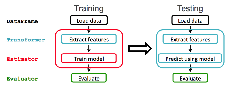
Image: https://mapr.com/blog/fast-data-processing-pipeline-predicting-flight-delays-using-apache-apis-pt-1/
We will use an ML Pipeline to pass the data through transformers in order to extract the features and an estimator to produce the model.
Transformer: A Transformer is an algorithm which transforms one DataFrame into another DataFrame. We will use a transformer to get a DataFrame with a features vector column.Estimator: An Estimator is an algorithm which can be fit on a DataFrame to produce a Transformer. We will use a an estimator to train a model which can transform data to get predictions.Pipeline: A Pipeline chains multiple Transformers and Estimators together to specify a ML workflow.
Feature Extraction and Pipelining
The ML package needs the label and feature vector to be added as columns to the input dataframe. We set up a pipeline to pass the data through transformers in order to extract the features and label. We use a StringIndexer to encode a string columns to a column of number indices. We use a OneHotEncoder to map a number indices column to a column of binary vectors, with at most a single one-value. Encoding categorical features allows machine learning algorithms to treat categorical features appropriately, improving performance. An example of StringIndexing and OneHotEncoding for 'race' is shown below:

5.1 Use a combination of StringIndexer and OneHotEncoder to encode Categorical columns:
Experiment: Let's StringIndex the 'race' column:
col_name = "race"
race_indexer_model = StringIndexer(inputCol=col_name, outputCol="{0}_indexed".format(col_name)).fit(train_df)
race_indexed_df = race_indexer_model.transform(train_df)
# check the encoded carrier values
race_indexer_model.labels
['White', 'Black', 'Asian-Pac-Islander', 'Amer-Indian-Eskimo', 'Other']
# check the race code and index mapping
race_indexed_df.select(['race', 'race_indexed']).distinct().show()
+------------------+------------+
|              race|race_indexed|
+------------------+------------+
|             Other|         4.0|
|             Black|         1.0|
|Amer-Indian-Eskimo|         3.0|
|Asian-Pac-Islander|         2.0|
|             White|         0.0|
+------------------+------------+
Experiment: Let's OneHotEncode the 'race' column:
pyspark.ml.feature.OneHotEncoder maps a column of category indices to a column of binary vectors, with at most a single one-value per row that indicates the input category index. For example with 5 categories, an input value of 2.0 would map to an output vector of [0.0, 0.0, 1.0, 0.0]. The last category is not included by default (configurable via dropLast=True) because it makes the vector entries sum up to one, and hence linearly dependent. So an input value of 4.0 maps to [0.0, 0.0, 0.0, 0.0]. Note that this is different from scikit-learn's OneHotEncoder, which keeps all categories. The output vectors are sparse. However, if we configure dropLast=False, then with 5 categories, an input value of 2.0 would map to an output vector of [0.0, 0.0, 1.0, 0.0, 0.0].
race_encoder = OneHotEncoder(inputCol="{0}_indexed".format(col_name), outputCol="{0}_encoded".format(col_name), dropLast=False)
race_encoded_df = race_encoder.transform(race_indexed_df)
(race_encoded_df
 .select('age', 'marital_status', 'race', 'race_indexed', 'race_encoded', 'income')
 .limit(10)
 .toPandas())
| age | marital_status | race | race_indexed | race_encoded | income | |
|---|---|---|---|---|---|---|
| 0 | 39 | Never-married | White | 0.0 | (1.0, 0.0, 0.0, 0.0, 0.0) | <=50K |
| 1 | 50 | Married-civ-spouse | White | 0.0 | (1.0, 0.0, 0.0, 0.0, 0.0) | <=50K |
| 2 | 38 | Divorced | White | 0.0 | (1.0, 0.0, 0.0, 0.0, 0.0) | <=50K |
| 3 | 53 | Married-civ-spouse | Black | 1.0 | (0.0, 1.0, 0.0, 0.0, 0.0) | <=50K |
| 4 | 28 | Married-civ-spouse | Black | 1.0 | (0.0, 1.0, 0.0, 0.0, 0.0) | <=50K |
| 5 | 37 | Married-civ-spouse | White | 0.0 | (1.0, 0.0, 0.0, 0.0, 0.0) | <=50K |
| 6 | 49 | Married-spouse-absent | Black | 1.0 | (0.0, 1.0, 0.0, 0.0, 0.0) | <=50K |
| 7 | 52 | Married-civ-spouse | White | 0.0 | (1.0, 0.0, 0.0, 0.0, 0.0) | >50K |
| 8 | 31 | Never-married | White | 0.0 | (1.0, 0.0, 0.0, 0.0, 0.0) | >50K |
| 9 | 42 | Married-civ-spouse | White | 0.0 | (1.0, 0.0, 0.0, 0.0, 0.0) | >50K |
Note: The column vector is a SparseVector: (5,[0],[1.0]) means there are 5 elements and the 0th position has a 1.0.
5.2 Combine StringIndexer, OneHotEncoder, StandardScaler, VectorAssembler put features into a feature vector column:
assembled_train_df = train_df
assembled_test_df = test_df
OneHotEncode all categorical columns:
# categorical columns
categorical_columns = ["workclass", "marital_status", "occupation", "relationship", "race", "sex", "native_country"]
# numerial columns
numerical_columns = ["age", "education_num", "capital_gain", "capital_loss", "hours_per_week"]
string_indexer_models = []
one_hot_encoders = []
for col_name in categorical_columns:
    # String Indexers will encode string categorical columns into a column of numeric indices
    string_indexer_model = StringIndexer(inputCol=col_name, outputCol="{0}_indexed".format(col_name)).fit(assembled_train_df)
    assembled_train_df = string_indexer_model.transform(assembled_train_df)
    assembled_test_df = string_indexer_model.transform(assembled_test_df)

    string_indexer_models.append(string_indexer_model)

    # OneHotEncoders map number indices column to column of binary vectors
    one_hot_encoder = OneHotEncoder(inputCol="{0}_indexed".format(col_name), outputCol="{0}_encoded".format(col_name), dropLast=False)
    assembled_train_df = one_hot_encoder.transform(assembled_train_df)
    assembled_test_df = one_hot_encoder.transform(assembled_test_df)

    one_hot_encoders.append(one_hot_encoder)
(assembled_train_df
 .select('age', 'marital_status_indexed', 'marital_status_encoded', 'race_indexed', 'race_encoded', 'income')
 .limit(10)
 .toPandas())
| age | marital_status_indexed | marital_status_encoded | race_indexed | race_encoded | income | |
|---|---|---|---|---|---|---|
| 0 | 39 | 1.0 | (0.0, 1.0, 0.0, 0.0, 0.0, 0.0, 0.0) | 0.0 | (1.0, 0.0, 0.0, 0.0, 0.0) | <=50K |
| 1 | 50 | 0.0 | (1.0, 0.0, 0.0, 0.0, 0.0, 0.0, 0.0) | 0.0 | (1.0, 0.0, 0.0, 0.0, 0.0) | <=50K |
| 2 | 38 | 2.0 | (0.0, 0.0, 1.0, 0.0, 0.0, 0.0, 0.0) | 0.0 | (1.0, 0.0, 0.0, 0.0, 0.0) | <=50K |
| 3 | 53 | 0.0 | (1.0, 0.0, 0.0, 0.0, 0.0, 0.0, 0.0) | 1.0 | (0.0, 1.0, 0.0, 0.0, 0.0) | <=50K |
| 4 | 28 | 0.0 | (1.0, 0.0, 0.0, 0.0, 0.0, 0.0, 0.0) | 1.0 | (0.0, 1.0, 0.0, 0.0, 0.0) | <=50K |
| 5 | 37 | 0.0 | (1.0, 0.0, 0.0, 0.0, 0.0, 0.0, 0.0) | 0.0 | (1.0, 0.0, 0.0, 0.0, 0.0) | <=50K |
| 6 | 49 | 5.0 | (0.0, 0.0, 0.0, 0.0, 0.0, 1.0, 0.0) | 1.0 | (0.0, 1.0, 0.0, 0.0, 0.0) | <=50K |
| 7 | 52 | 0.0 | (1.0, 0.0, 0.0, 0.0, 0.0, 0.0, 0.0) | 0.0 | (1.0, 0.0, 0.0, 0.0, 0.0) | >50K |
| 8 | 31 | 1.0 | (0.0, 1.0, 0.0, 0.0, 0.0, 0.0, 0.0) | 0.0 | (1.0, 0.0, 0.0, 0.0, 0.0) | >50K |
| 9 | 42 | 0.0 | (1.0, 0.0, 0.0, 0.0, 0.0, 0.0, 0.0) | 0.0 | (1.0, 0.0, 0.0, 0.0, 0.0) | >50K |
StandardScale all numerical columns:
Standardize all the numerical columns of the Spark DataFrame. StandardScaler expects all the numerical columns in a vectorized form. Hence we need a VectorAssembler to transform all the numerical features into a Vectorized feature column.
# Vectorize the numerical features first
scaler_vector_assembler = VectorAssembler(inputCols=numerical_columns, outputCol="numerical_features")
assembled_train_df = scaler_vector_assembler.transform(assembled_train_df)
assembled_test_df = scaler_vector_assembler.transform(assembled_test_df)
(assembled_train_df
 .select('numerical_features', 'marital_status_encoded', 'race_encoded', 'income')
 .limit(10)
 .toPandas())
| numerical_features | marital_status_encoded | race_encoded | income | |
|---|---|---|---|---|
| 0 | [39.0, 13.0, 2174.0, 0.0, 40.0] | (0.0, 1.0, 0.0, 0.0, 0.0, 0.0, 0.0) | (1.0, 0.0, 0.0, 0.0, 0.0) | <=50K |
| 1 | [50.0, 13.0, 0.0, 0.0, 13.0] | (1.0, 0.0, 0.0, 0.0, 0.0, 0.0, 0.0) | (1.0, 0.0, 0.0, 0.0, 0.0) | <=50K |
| 2 | [38.0, 9.0, 0.0, 0.0, 40.0] | (0.0, 0.0, 1.0, 0.0, 0.0, 0.0, 0.0) | (1.0, 0.0, 0.0, 0.0, 0.0) | <=50K |
| 3 | [53.0, 7.0, 0.0, 0.0, 40.0] | (1.0, 0.0, 0.0, 0.0, 0.0, 0.0, 0.0) | (0.0, 1.0, 0.0, 0.0, 0.0) | <=50K |
| 4 | [28.0, 13.0, 0.0, 0.0, 40.0] | (1.0, 0.0, 0.0, 0.0, 0.0, 0.0, 0.0) | (0.0, 1.0, 0.0, 0.0, 0.0) | <=50K |
| 5 | [37.0, 14.0, 0.0, 0.0, 40.0] | (1.0, 0.0, 0.0, 0.0, 0.0, 0.0, 0.0) | (1.0, 0.0, 0.0, 0.0, 0.0) | <=50K |
| 6 | [49.0, 5.0, 0.0, 0.0, 16.0] | (0.0, 0.0, 0.0, 0.0, 0.0, 1.0, 0.0) | (0.0, 1.0, 0.0, 0.0, 0.0) | <=50K |
| 7 | [52.0, 9.0, 0.0, 0.0, 45.0] | (1.0, 0.0, 0.0, 0.0, 0.0, 0.0, 0.0) | (1.0, 0.0, 0.0, 0.0, 0.0) | >50K |
| 8 | [31.0, 14.0, 14084.0, 0.0, 50.0] | (0.0, 1.0, 0.0, 0.0, 0.0, 0.0, 0.0) | (1.0, 0.0, 0.0, 0.0, 0.0) | >50K |
| 9 | [42.0, 13.0, 5178.0, 0.0, 40.0] | (1.0, 0.0, 0.0, 0.0, 0.0, 0.0, 0.0) | (1.0, 0.0, 0.0, 0.0, 0.0) | >50K |
Observe how all the numerical features have been clubbed as vectors into a single column.
# create StandardScalerModel
standard_scaler_model = StandardScaler(withMean=True, inputCol='numerical_features', outputCol='numerical_features_scaled').fit(assembled_train_df)
# apply StandardScaler
assembled_train_df = standard_scaler_model.transform(assembled_train_df)
assembled_test_df = standard_scaler_model.transform(assembled_test_df)
assembled_train_df.select('numerical_features_scaled', 'marital_status_encoded', 'race_encoded', 'income').limit(10).toPandas()
| numerical_features_scaled | marital_status_encoded | race_encoded | income | |
|---|---|---|---|---|
| 0 | [0.03067008638, 1.13472133885, 0.148450615588, -0.216656200028, -0.0354289029213] | (0.0, 1.0, 0.0, 0.0, 0.0, 0.0, 0.0) | (1.0, 0.0, 0.0, 0.0, 0.0) | <=50K |
| 1 | [0.837096125788, 1.13472133885, -0.145918242817, -0.216656200028, -2.22211899816] | (1.0, 0.0, 0.0, 0.0, 0.0, 0.0, 0.0) | (1.0, 0.0, 0.0, 0.0, 0.0) | <=50K |
| 2 | [-0.042641371748, -0.420053173618, -0.145918242817, -0.216656200028, -0.0354289029213] | (0.0, 0.0, 1.0, 0.0, 0.0, 0.0, 0.0) | (1.0, 0.0, 0.0, 0.0, 0.0) | <=50K |
| 3 | [1.05703050017, -1.19744042985, -0.145918242817, -0.216656200028, -0.0354289029213] | (1.0, 0.0, 0.0, 0.0, 0.0, 0.0, 0.0) | (0.0, 1.0, 0.0, 0.0, 0.0) | <=50K |
| 4 | [-0.775755953028, 1.13472133885, -0.145918242817, -0.216656200028, -0.0354289029213] | (1.0, 0.0, 0.0, 0.0, 0.0, 0.0, 0.0) | (0.0, 1.0, 0.0, 0.0, 0.0) | <=50K |
| 5 | [-0.115952829876, 1.52341496696, -0.145918242817, -0.216656200028, -0.0354289029213] | (1.0, 0.0, 0.0, 0.0, 0.0, 0.0, 0.0) | (1.0, 0.0, 0.0, 0.0, 0.0) | <=50K |
| 6 | [0.76378466766, -1.97482768608, -0.145918242817, -0.216656200028, -1.97915343202] | (0.0, 0.0, 0.0, 0.0, 0.0, 1.0, 0.0) | (0.0, 1.0, 0.0, 0.0, 0.0) | <=50K |
| 7 | [0.983719042044, -0.420053173618, -0.145918242817, -0.216656200028, 0.369513707308] | (1.0, 0.0, 0.0, 0.0, 0.0, 0.0, 0.0) | (1.0, 0.0, 0.0, 0.0, 0.0) | >50K |
| 8 | [-0.555821578644, 1.52341496696, 1.76111533666, -0.216656200028, 0.774456317537] | (0.0, 1.0, 0.0, 0.0, 0.0, 0.0, 0.0) | (1.0, 0.0, 0.0, 0.0, 0.0) | >50K |
| 9 | [0.250604460764, 1.13472133885, 0.55520500871, -0.216656200028, -0.0354289029213] | (1.0, 0.0, 0.0, 0.0, 0.0, 0.0, 0.0) | (1.0, 0.0, 0.0, 0.0, 0.0) | >50K |
Observation: toPandas() method transforms the Sparse One Hot Encoded Vectors into DenseVectors for display.
Transform Income attribute into Binary Labels:
income_indexer_model = StringIndexer(inputCol='income', outputCol='label').fit(assembled_train_df)
income_indexer_model.labels
['<=50K', '>50K']
assembled_train_df = income_indexer_model.transform(assembled_train_df)
assembled_test_df = income_indexer_model.transform(assembled_test_df)
# check the income level and index mapping
assembled_train_df.select(["income", "label"]).distinct().toPandas()
| income | label | |
|---|---|---|
| 0 | <=50K | 0.0 |
| 1 | >50K | 1.0 |
(assembled_train_df
 .select('numerical_features_scaled', 'marital_status_encoded', 'race_encoded', 'income', 'label')
 .limit(10)
 .toPandas())
| numerical_features_scaled | marital_status_encoded | race_encoded | income | label | |
|---|---|---|---|---|---|
| 0 | [0.03067008638, 1.13472133885, 0.148450615588, -0.216656200028, -0.0354289029213] | (0.0, 1.0, 0.0, 0.0, 0.0, 0.0, 0.0) | (1.0, 0.0, 0.0, 0.0, 0.0) | <=50K | 0.0 |
| 1 | [0.837096125788, 1.13472133885, -0.145918242817, -0.216656200028, -2.22211899816] | (1.0, 0.0, 0.0, 0.0, 0.0, 0.0, 0.0) | (1.0, 0.0, 0.0, 0.0, 0.0) | <=50K | 0.0 |
| 2 | [-0.042641371748, -0.420053173618, -0.145918242817, -0.216656200028, -0.0354289029213] | (0.0, 0.0, 1.0, 0.0, 0.0, 0.0, 0.0) | (1.0, 0.0, 0.0, 0.0, 0.0) | <=50K | 0.0 |
| 3 | [1.05703050017, -1.19744042985, -0.145918242817, -0.216656200028, -0.0354289029213] | (1.0, 0.0, 0.0, 0.0, 0.0, 0.0, 0.0) | (0.0, 1.0, 0.0, 0.0, 0.0) | <=50K | 0.0 |
| 4 | [-0.775755953028, 1.13472133885, -0.145918242817, -0.216656200028, -0.0354289029213] | (1.0, 0.0, 0.0, 0.0, 0.0, 0.0, 0.0) | (0.0, 1.0, 0.0, 0.0, 0.0) | <=50K | 0.0 |
| 5 | [-0.115952829876, 1.52341496696, -0.145918242817, -0.216656200028, -0.0354289029213] | (1.0, 0.0, 0.0, 0.0, 0.0, 0.0, 0.0) | (1.0, 0.0, 0.0, 0.0, 0.0) | <=50K | 0.0 |
| 6 | [0.76378466766, -1.97482768608, -0.145918242817, -0.216656200028, -1.97915343202] | (0.0, 0.0, 0.0, 0.0, 0.0, 1.0, 0.0) | (0.0, 1.0, 0.0, 0.0, 0.0) | <=50K | 0.0 |
| 7 | [0.983719042044, -0.420053173618, -0.145918242817, -0.216656200028, 0.369513707308] | (1.0, 0.0, 0.0, 0.0, 0.0, 0.0, 0.0) | (1.0, 0.0, 0.0, 0.0, 0.0) | >50K | 1.0 |
| 8 | [-0.555821578644, 1.52341496696, 1.76111533666, -0.216656200028, 0.774456317537] | (0.0, 1.0, 0.0, 0.0, 0.0, 0.0, 0.0) | (1.0, 0.0, 0.0, 0.0, 0.0) | >50K | 1.0 |
| 9 | [0.250604460764, 1.13472133885, 0.55520500871, -0.216656200028, -0.0354289029213] | (1.0, 0.0, 0.0, 0.0, 0.0, 0.0, 0.0) | (1.0, 0.0, 0.0, 0.0, 0.0) | >50K | 1.0 |
Assemble transformed features into one Feature Vector for Spark:
feature_cols = ["{0}_encoded".format(col) for col in categorical_columns] + ['numerical_features_scaled']
feature_cols
['workclass_encoded',
 'marital_status_encoded',
 'occupation_encoded',
 'relationship_encoded',
 'race_encoded',
 'sex_encoded',
 'native_country_encoded',
 'numerical_features_scaled']
# The VectorAssembler combines a given list of columns into a single feature vector column.
feature_assembler = VectorAssembler(inputCols=feature_cols, outputCol="features")
# cache the dataframe because we would be reusing this again and again
assembled_train_df = feature_assembler.transform(assembled_train_df).cache()
assembled_test_df = feature_assembler.transform(assembled_test_df).cache()
assembled_train_df.columns
['age',
 'workclass',
 'fnlgwt',
 'education_num',
 'marital_status',
 'occupation',
 'relationship',
 'race',
 'sex',
 'capital_gain',
 'capital_loss',
 'hours_per_week',
 'native_country',
 'income',
 'workclass_indexed',
 'workclass_encoded',
 'marital_status_indexed',
 'marital_status_encoded',
 'occupation_indexed',
 'occupation_encoded',
 'relationship_indexed',
 'relationship_encoded',
 'race_indexed',
 'race_encoded',
 'sex_indexed',
 'sex_encoded',
 'native_country_indexed',
 'native_country_encoded',
 'numerical_features',
 'numerical_features_scaled',
 'label',
 'features']
Result: SparseVector representation of the Feature Vectors
assembled_train_df.select('features', 'label').limit(5).show(10,100)
+----------------------------------------------------------------------------------------------------+-----+
|                                                                                            features|label|
+----------------------------------------------------------------------------------------------------+-----+
|(91,[4,10,19,32,37,42,44,86,87,88,89,90],[1.0,1.0,1.0,1.0,1.0,1.0,1.0,0.03067008637999638,1.13472...|  0.0|
|(91,[1,9,18,31,37,42,44,86,87,88,89,90],[1.0,1.0,1.0,1.0,1.0,1.0,1.0,0.8370961257882483,1.1347213...|  0.0|
|(91,[0,11,25,32,37,42,44,86,87,88,89,90],[1.0,1.0,1.0,1.0,1.0,1.0,1.0,-0.04264137174802653,-0.420...|  0.0|
|(91,[0,9,25,31,38,42,44,86,87,88,89,90],[1.0,1.0,1.0,1.0,1.0,1.0,1.0,1.057030500172317,-1.1974404...|  0.0|
|(91,[0,9,16,35,38,43,53,86,87,88,89,90],[1.0,1.0,1.0,1.0,1.0,1.0,1.0,-0.7757559530282556,1.134721...|  0.0|
+----------------------------------------------------------------------------------------------------+-----+
7. Class Imbalance
Let's see the distribution of negative and positive classes in our training dataset.
(assembled_train_df
 .groupBy('income')
 .count()
 .withColumn('%age', F.round(col('count') / assembled_train_df.count(), 2))
 .toPandas())
| income | count | %age | |
|---|---|---|---|
| 0 | <=50K | 24720 | 0.76 |
| 1 | >50K | 7841 | 0.24 |
There is quite a significant class imbalance. In order to ensure that our model is sensitive to the income levels, we can put the two sample types on the same footing. In this case we have 76% negatives (label == 0) and 24% positives (label == 1) and in the dataset, so theoretically we want to "under-sample" the negative class. The logistic loss objective function should treat the positive class (label == 1) with higher weight.
https://stackoverflow.com/questions/33372838/dealing-with-unbalanced-datasets-in-spark-mllib
7.1 Assign class_weights to class labels:
We add a new column to the dataframe for each record in the dataset:
label1count = assembled_train_df.filter(col('income') == '>50K').count()
datacount = assembled_train_df.count()
weight_balance = np.round((datacount - label1count) / datacount, decimals=2)
weight_balance
0.76000000000000001
# we "under sample" the negative class
assembled_train_df = (assembled_train_df
                      .withColumn('class_weight',
                            F.when(col('income') == '>50K', F.lit(weight_balance)).otherwise(F.lit(1 - weight_balance)))
                     )
assembled_train_df.select('class_weight', 'label').limit(20).toPandas()
| class_weight | label | |
|---|---|---|
| 0 | 0.24 | 0.0 |
| 1 | 0.24 | 0.0 |
| 2 | 0.24 | 0.0 |
| 3 | 0.24 | 0.0 |
| 4 | 0.24 | 0.0 |
| 5 | 0.24 | 0.0 |
| 6 | 0.24 | 0.0 |
| 7 | 0.76 | 1.0 |
| 8 | 0.76 | 1.0 |
| 9 | 0.76 | 1.0 |
| 10 | 0.76 | 1.0 |
| 11 | 0.76 | 1.0 |
| 12 | 0.24 | 0.0 |
| 13 | 0.24 | 0.0 |
| 14 | 0.76 | 1.0 |
| 15 | 0.24 | 0.0 |
| 16 | 0.24 | 0.0 |
| 17 | 0.24 | 0.0 |
| 18 | 0.24 | 0.0 |
| 19 | 0.76 | 1.0 |
We will use this class_weight column when we define our LogisticRegression model.
8. Stratified Sampling
We need to ensure that when we create the training and validation set the two different class labels are represented in the same proportion in the training and the validation set. This is known as stratified sampling. The data is split using the proportion of the class labels.
The DataFrames sampleBy() function provides a way of specifying fractions of each sample type to be returned.
We will split the training set into training and validation set in the ratio 0.75:0.25. So we will take 25% from each class to create the validation set and the rest 75% from each class would go in the training set.
(assembled_train_df
 .groupBy('income')
 .count()
 .withColumn('%age', F.round(col('count') / assembled_train_df.count(), 2))
 .toPandas())
| income | count | %age | |
|---|---|---|---|
| 0 | <=50K | 24720 | 0.76 |
| 1 | >50K | 7841 | 0.24 |
# specify the exact fraction desired from each key as a dictionary
fractions = {0.0: 0.25, 1.0: 0.25}
# create the validation set with 25% of the entire data and same distribution of income levels
assembled_validation_df = assembled_train_df.stat.sampleBy('label', fractions, seed=rnd_seed).cache()
# subtract the validation set from the original training set to get 75% of the entire data
# and same distribution of income levels
assembled_train_df = assembled_train_df.subtract(assembled_validation_df).cache()
Recheck the distribution:
Check whether the training and validation set contain rows across are represented in the same proportion of income levels.
(assembled_train_df
 .groupBy('income')
 .count()
 .withColumn('%age', F.round(col('count') / assembled_train_df.count(), 2))
 .toPandas())
| income | count | %age | |
|---|---|---|---|
| 0 | <=50K | 18414 | 0.76 |
| 1 | >50K | 5851 | 0.24 |
(assembled_validation_df
 .groupBy('income')
 .count()
 .withColumn('%age', F.round(col('count') / assembled_validation_df.count(), 2))
 .toPandas())
| income | count | %age | |
|---|---|---|---|
| 0 | <=50K | 6284 | 0.76 |
| 1 | >50K | 1988 | 0.24 |
9. Train a Logistic Regression
We will create a LogisticRegression model with class_weight specified.
# watch how we specify the class_weight using the weightCol feature
log_reg = LogisticRegression(featuresCol='features', labelCol='label', weightCol='class_weight', maxIter=20, family='binomial')
evaluator = BinaryClassificationEvaluator(rawPredictionCol='rawPrediction', labelCol='label', metricName='areaUnderROC')
model = log_reg.fit(assembled_train_df)
train_preds = model.transform(assembled_validation_df)
print(train_preds.columns)
['age', 'workclass', 'fnlgwt', 'education_num', 'marital_status', 'occupation', 'relationship', 'race', 'sex', 'capital_gain', 'capital_loss', 'hours_per_week', 'native_country', 'income', 'workclass_indexed', 'workclass_encoded', 'marital_status_indexed', 'marital_status_encoded', 'occupation_indexed', 'occupation_encoded', 'relationship_indexed', 'relationship_encoded', 'race_indexed', 'race_encoded', 'sex_indexed', 'sex_encoded', 'native_country_indexed', 'native_country_encoded', 'numerical_features', 'numerical_features_scaled', 'label', 'features', 'class_weight', 'rawPrediction', 'probability', 'prediction']
train_areaUnderROC = evaluator.evaluate(train_preds)
train_areaUnderROC
0.9127818710480433
trainpredlbls = train_preds.select("prediction", "label").cache()
trainpredlbls.limit(10).toPandas()
| prediction | label | |
|---|---|---|
| 0 | 0.0 | 0.0 |
| 1 | 1.0 | 1.0 |
| 2 | 1.0 | 1.0 |
| 3 | 1.0 | 1.0 |
| 4 | 0.0 | 0.0 |
| 5 | 0.0 | 1.0 |
| 6 | 1.0 | 1.0 |
| 7 | 0.0 | 0.0 |
| 8 | 0.0 | 0.0 |
| 9 | 0.0 | 1.0 |
Training Accuracy:
def accuracy(predlbls):
    counttotal = predlbls.count()
    correct = predlbls.filter(col('label') == col("prediction")).count()
    wrong = predlbls.filter(col('label') != col("prediction")).count()
    ratioCorrect = float(correct)/counttotal
    print("Correct: {0}, Wrong: {1}, Model Accuracy: {2}".format(correct, wrong, np.round(ratioCorrect, 2)))
accuracy(trainpredlbls)
Correct: 6750, Wrong: 1522, Model Accuracy: 0.82
Training & Validation Accuracy: Using Spark 2.3.0 enhancements:
Spark 2.3.0 has introdcued several new methods in BinaryLogisticRegressionSummary which we can leverage to get various metrics.
train_summary = model.evaluate(assembled_train_df)
validation_summary = model.evaluate(assembled_validation_df)
type(train_summary), type(validation_summary)
(pyspark.ml.classification.BinaryLogisticRegressionSummary,
 pyspark.ml.classification.BinaryLogisticRegressionSummary)
print('Training Accuracy   :', train_summary.accuracy)
print('Validation Accuracy :', validation_summary.accuracy)
Training Accuracy   : 0.8091901916340408
Validation Accuracy : 0.8160058027079303
train_summary.areaUnderROC
validation_summary.areaUnderROC
0.906075974495489
0.9128234156690619
validation_summary.fMeasureByLabel(beta=1.0)
[0.8684301521438451, 0.6941318327974276]
validation_summary.precisionByLabel
[0.9506056018168054, 0.5779785809906292]
validation_summary.recallByLabel
[0.7993316359007002, 0.8687122736418511]
Null Accuracy:
Our model should at least perform better than the Null Accuracy. Null Accuracy is defined as the accuracy we would have got if we would have blindly predicted the majority class of the training set as the label.
train_total = trainpredlbls.count()
train_label0count = trainpredlbls.filter(col("label") == 0.0).count()
train_label1count = trainpredlbls.filter(col("label") == 1.0).count()
# If we would have predicted everything to be the majority label then what would have been the accuracy
max(train_label0count, train_label1count) / train_total
0.7596711798839458
Observation: The model accuracy on the training set is 0.85 i.e. it is at least doing better than the NULL accuracy.
Test Accuracy:
test_preds = model.transform(assembled_test_df)
test_areaUnderROC = evaluator.evaluate(test_preds)
test_areaUnderROC
0.9030185356992586
testpredlbls = test_preds.select("prediction", "label")
accuracy(testpredlbls)
Correct: 13122, Wrong: 3159, Model Accuracy: 0.81
Using Spark 2.3.0 enhancements:
test_summary = model.evaluate(assembled_test_df)
type(test_summary)
pyspark.ml.classification.BinaryLogisticRegressionSummary
test_summary.accuracy
0.8059701492537313
test_summary.areaUnderROC
0.9029399680209164
test_summary.fMeasureByLabel(beta=1.0)
[0.862274926973885, 0.6717922077922077]
test_summary.precisionByLabel
[0.9416301656827271, 0.5594393493684028]
test_summary.recallByLabel
[0.7952553277040612, 0.8406136245449818]
test_summary.roc.limit(10).toPandas()
| FPR | TPR | |
|---|---|---|
| 0 | 0.000000 | 0.000000 |
| 1 | 0.000080 | 0.050962 |
| 2 | 0.000161 | 0.089444 |
| 3 | 0.000885 | 0.126105 |
| 4 | 0.002091 | 0.161206 |
| 5 | 0.004021 | 0.193968 |
| 6 | 0.006112 | 0.226989 |
| 7 | 0.008203 | 0.261050 |
| 8 | 0.011017 | 0.292512 |
| 9 | 0.014395 | 0.324493 |
train_roc_pdf = train_summary.roc.toPandas()
validation_roc_pdf = validation_summary.roc.toPandas()
test_roc_pdf = test_summary.roc.toPandas()
plt.figure(figsize=(6,4))
plt.plot(train_roc_pdf['FPR'], train_roc_pdf['TPR'], lw=1, label='Train AUC = %0.2f' % (train_summary.areaUnderROC))
plt.plot(validation_roc_pdf['FPR'], validation_roc_pdf['TPR'], lw=1, label='Validation AUC = %0.2f' % (test_summary.areaUnderROC))
plt.plot(test_roc_pdf['FPR'], test_roc_pdf['TPR'], lw=1, label='Test AUC = %0.2f' % (validation_summary.areaUnderROC))
plt.plot([0, 1], [0, 1], '--', color=(0.6, 0.6, 0.6), label='NULL Accuracy')
plt.title('ROC AUC Curve')
plt.legend();

10. Setup a pipeline with feature transformers and model estimator
Since, we have now trained a model after feature transformation, we are now in a position to set up a pipeline that will call feature extractors, transformers, assemblers, estimator in a chain automatically.
# categorical columns
categorical_columns = ["workclass", "marital_status", "occupation", "relationship", "race", "sex", "native_country"]
# numerial columns
numerical_columns = ["age", "education_num", "capital_gain", "capital_loss", "hours_per_week"]
# String Indexers will encode string categorical columns into a column of numeric indices
string_indexers = [StringIndexer(inputCol=col_name, outputCol="{0}_indexed".format(col_name), handleInvalid='skip') for col_name in categorical_columns]
In our training set there is a single row where the native_country has value 'Holand-Netherlans'. That single will fall into a training or test fold during cross validation leading to Spark throwing an exception saying that it has encountered an unseen value. In order to skip that record during cross-validation we need to configure handleInvalid='skip'.
More details here: http://spark.apache.org/docs/2.3.0/api/python/pyspark.ml.html#pyspark.ml.feature.StringIndexer
# OneHotEncoders map number indices column to column of binary vectors
one_hot_encoders = [OneHotEncoder(inputCol="{0}_indexed".format(col_name), outputCol="{0}_encoded".format(col_name), dropLast=False) for col_name in categorical_columns]
scaler_vector_assembler = VectorAssembler(inputCols=numerical_columns, outputCol="numerical_features")
standard_scaler = StandardScaler(withMean=True, inputCol='numerical_features', outputCol='numerical_features_scaled')
income_indexer = StringIndexer(inputCol='income', outputCol='label')
feature_cols = ["{0}_encoded".format(col) for col in categorical_columns] + ['numerical_features_scaled']
feature_cols
['workclass_encoded',
 'marital_status_encoded',
 'occupation_encoded',
 'relationship_encoded',
 'race_encoded',
 'sex_encoded',
 'native_country_encoded',
 'numerical_features_scaled']
# The VectorAssembler combines a given list of columns into a single feature vector column.
feature_assembler = VectorAssembler(inputCols=feature_cols, outputCol="features")
log_reg = LogisticRegression(featuresCol='features', labelCol='label', weightCol='class_weight', maxIter=20, family='binomial')
Assemble the pipeline:
steps = string_indexers + one_hot_encoders + [scaler_vector_assembler, standard_scaler, income_indexer, feature_assembler, log_reg]
steps
[StringIndexer_492880a800b95ea8119e,
 StringIndexer_464080636b53dfa4e597,
 StringIndexer_424b81a8c7a59e5f5aba,
 StringIndexer_45e39b2235e6957f74d7,
 StringIndexer_4a8b8d8e9d52eb2aa17d,
 StringIndexer_40ee835b624f551c2ee1,
 StringIndexer_41398d95da8dc65bd9c8,
 OneHotEncoder_4973918c918af3986164,
 OneHotEncoder_4ecaa69d59f4695b2ba8,
 OneHotEncoder_40d4958687354e951eb7,
 OneHotEncoder_444195b4f6d6f3fa5d51,
 OneHotEncoder_413c976fbef74af7ecdf,
 OneHotEncoder_4836bed3a623d4ad42c7,
 OneHotEncoder_437384bdd331db933a39,
 VectorAssembler_45f197169aec013291b7,
 StandardScaler_4d528f4f1c75958f9bc5,
 StringIndexer_4083a3b050fd3ad394a6,
 VectorAssembler_4ed58472c709978bc1cd,
 LogisticRegression_41a2ada033060e643027]
pipeline = Pipeline(stages=steps)
11. Set up a CrossValidator with the Parameters, a Logistic Regressor estimator and a BinaryClassificationEvaluator
A common technique for model selection is k-fold cross-validation, where the data is randomly split into k partitions. Each partition is used once as the testing dataset, while the rest k - 1 are used for the training. k Models are then generated using the training sets and evaluated with the testing sets, resulting in k model performance measurements.
We can also provide a grid of paramater names and a set of values for each paramater that can be tried to see which set of parameter values of the logistic regression produce the best model.
Spark ML supports k-fold cross-validation with a transformation/estimation pipeline to try out different combinations of parameters, using the grid search process. Here, we set up the parameters to test, and a cross-validation evaluator to construct a model selection workflow.
We use a ParamGridBuilder to construct the parameter grid. We define an BinaryClassificationEvaluator, which will evaluate the model by comparing the test label column with the test prediction column. We use a CrossValidator with 5 folds for model selection.
The model parameters leading to the highest performance metric produce the best model.
11.1 Set up a Grid of Parameters to tune
# set param grid to search through logistic regression's regularization parameter for best model
paramGrid = (ParamGridBuilder()
             .addGrid(log_reg.regParam, [0.1, 0.01, 0.001])
             .addGrid(log_reg.elasticNetParam, [0.0, 0.5, 1.0])
             .build())
evaluator = BinaryClassificationEvaluator(rawPredictionCol='rawPrediction', labelCol='label', metricName='areaUnderROC')
# Set up 5-fold cross validation with paramGrid
crossVal = CrossValidator(estimator=pipeline, evaluator=evaluator, estimatorParamMaps=paramGrid, numFolds=5)
The CrossValidator uses the Estimator Pipeline, the Parameter Grid, and the Classification Evaluator to fit the training data set and returns a model.
11.2 Use CrossValidator Estimator to fit the training data set
Add the class_weight column before we invoke the cross_validator:
# we "under sample" the negative class
train_df = (train_df.withColumn('class_weight',
                    F.when(col('income') == '>50K', F.lit(weight_balance)).otherwise(F.lit(1 - weight_balance))))
cvModel = crossVal.fit(train_df)
The CrossValidator uses the ParamGridBuilder to iterate through the regParam parameter of the logistic regression and evaluate the models, repeating 5 times per parameter value for reliable results.
cvModel.bestModel.stages
[StringIndexer_492880a800b95ea8119e,
 StringIndexer_464080636b53dfa4e597,
 StringIndexer_424b81a8c7a59e5f5aba,
 StringIndexer_45e39b2235e6957f74d7,
 StringIndexer_4a8b8d8e9d52eb2aa17d,
 StringIndexer_40ee835b624f551c2ee1,
 StringIndexer_41398d95da8dc65bd9c8,
 OneHotEncoder_4973918c918af3986164,
 OneHotEncoder_4ecaa69d59f4695b2ba8,
 OneHotEncoder_40d4958687354e951eb7,
 OneHotEncoder_444195b4f6d6f3fa5d51,
 OneHotEncoder_413c976fbef74af7ecdf,
 OneHotEncoder_4836bed3a623d4ad42c7,
 OneHotEncoder_437384bdd331db933a39,
 VectorAssembler_45f197169aec013291b7,
 StandardScaler_4d528f4f1c75958f9bc5,
 StringIndexer_4083a3b050fd3ad394a6,
 VectorAssembler_4ed58472c709978bc1cd,
 LogisticRegression_41a2ada033060e643027]
# the last stage of the best model is the best logistic regressor
cvModel.bestModel.stages[-1]
LogisticRegression_41a2ada033060e643027
11.3 Get the Best Logistic Regression Model
best_log_reg_model = cvModel.bestModel.stages[-1]
best_log_reg_model
LogisticRegression_41a2ada033060e643027
# Extracts the embedded default param values and user-supplied values and then merges them into a flat param map
# with ordering: default param values < user-supplied values < extra.
best_log_reg_model.extractParamMap()
{Param(parent='LogisticRegression_41a2ada033060e643027', name='family', doc='The name of family which is a description of the label distribution to be used in the model. Supported options: auto, binomial, multinomial.'): 'binomial',
 Param(parent='LogisticRegression_41a2ada033060e643027', name='rawPredictionCol', doc='raw prediction (a.k.a. confidence) column name'): 'rawPrediction',
 Param(parent='LogisticRegression_41a2ada033060e643027', name='featuresCol', doc='features column name'): 'features',
 Param(parent='LogisticRegression_41a2ada033060e643027', name='elasticNetParam', doc='the ElasticNet mixing parameter, in range [0, 1]. For alpha = 0, the penalty is an L2 penalty. For alpha = 1, it is an L1 penalty'): 1.0,
 Param(parent='LogisticRegression_41a2ada033060e643027', name='fitIntercept', doc='whether to fit an intercept term'): True,
 Param(parent='LogisticRegression_41a2ada033060e643027', name='labelCol', doc='label column name'): 'label',
 Param(parent='LogisticRegression_41a2ada033060e643027', name='predictionCol', doc='prediction column name'): 'prediction',
 Param(parent='LogisticRegression_41a2ada033060e643027', name='threshold', doc='threshold in binary classification prediction, in range [0, 1]'): 0.5,
 Param(parent='LogisticRegression_41a2ada033060e643027', name='maxIter', doc='maximum number of iterations (>= 0)'): 20,
 Param(parent='LogisticRegression_41a2ada033060e643027', name='standardization', doc='whether to standardize the training features before fitting the model'): True,
 Param(parent='LogisticRegression_41a2ada033060e643027', name='weightCol', doc='weight column name. If this is not set or empty, we treat all instance weights as 1.0'): 'class_weight',
 Param(parent='LogisticRegression_41a2ada033060e643027', name='aggregationDepth', doc='suggested depth for treeAggregate (>= 2)'): 2,
 Param(parent='LogisticRegression_41a2ada033060e643027', name='regParam', doc='regularization parameter (>= 0)'): 0.001,
 Param(parent='LogisticRegression_41a2ada033060e643027', name='probabilityCol', doc='Column name for predicted class conditional probabilities. Note: Not all models output well-calibrated probability estimates! These probabilities should be treated as confidences, not precise probabilities'): 'probability',
 Param(parent='LogisticRegression_41a2ada033060e643027', name='tol', doc='the convergence tolerance for iterative algorithms (>= 0)'): 1e-06}
# Explains a single param and returns its name, doc, and optional default value and user-supplied value in a string.
for param in ['regParam', 'elasticNetParam', 'maxIter', 'tol']:
    best_log_reg_model.explainParam(param)
'regParam: regularization parameter (>= 0) (default: 0.0, current: 0.001)'
'elasticNetParam: the ElasticNet mixing parameter, in range [0, 1]. For alpha = 0, the penalty is an L2 penalty. For alpha = 1, it is an L1 penalty (default: 0.0, current: 1.0)'
'maxIter: maximum number of iterations (>= 0) (default: 100, current: 20)'
'tol: the convergence tolerance for iterative algorithms (>= 0) (default: 1e-06)'
11.4 Hyperparameter Heat Map
Next, we perform a visualization of hyperparameter search. Specifically, we create a heat map where the brighter colors correspond to higher areaUnderROC values.
grid_score_param_records = []
for metric, param_map in zip(cvModel.avgMetrics, paramGrid):
    grid_score_param_records.append(list(param_map.values()) + [metric])
grid_score_param_df = pd.DataFrame.from_records(grid_score_param_records, columns=['regParam', 'elasticNetParam', 'areaUnderROC'])
grid_score_param_df
| regParam | elasticNetParam | areaUnderROC | |
|---|---|---|---|
| 0 | 0.100 | 0.0 | 0.892122 |
| 1 | 0.100 | 0.5 | 0.870795 |
| 2 | 0.100 | 1.0 | 0.850399 |
| 3 | 0.010 | 0.0 | 0.901424 |
| 4 | 0.010 | 0.5 | 0.901224 |
| 5 | 0.010 | 1.0 | 0.900640 |
| 6 | 0.001 | 0.0 | 0.905587 |
| 7 | 0.001 | 0.5 | 0.906075 |
| 8 | 0.001 | 1.0 | 0.906433 |
grid_score_param_df = pd.pivot_table(grid_score_param_df, index=['regParam', 'elasticNetParam'], values=['areaUnderROC'])
grid_score_param_df
| areaUnderROC | ||
|---|---|---|
| regParam | elasticNetParam | |
| 0.001 | 0.0 | 0.905587 |
| 0.5 | 0.906075 | |
| 1.0 | 0.906433 | |
| 0.010 | 0.0 | 0.901424 |
| 0.5 | 0.901224 | |
| 1.0 | 0.900640 | |
| 0.100 | 0.0 | 0.892122 |
| 0.5 | 0.870795 | |
| 1.0 | 0.850399 |
grid_score_param_df['areaUnderROC'].unstack()
| elasticNetParam | 0.0 | 0.5 | 1.0 |
|---|---|---|---|
| regParam | |||
| 0.001 | 0.905587 | 0.906075 | 0.906433 |
| 0.010 | 0.901424 | 0.901224 | 0.900640 |
| 0.100 | 0.892122 | 0.870795 | 0.850399 |
# Compute the heat map
hmap = grid_score_param_df['areaUnderROC'].unstack()

# Set up the matplotlib figure
plt.figure(figsize=(6,4))
plt.title('Heat Map of Grid Search Parameters')
sns.heatmap(hmap, square=False, annot=True, cmap='viridis', fmt='.4g', linewidths=1);

12. Evaluate the best Logistic Regression Model
Training Accuracy - Using Spark 2.3.0 enhancements:
cv_train_summary = best_log_reg_model.summary
type(cv_train_summary)
pyspark.ml.classification.BinaryLogisticRegressionTrainingSummary
cv_train_summary.accuracy
0.8108166211111453
cv_train_summary.areaUnderROC
0.9077689352994321
cv_train_summary.fMeasureByLabel(beta=1.0)
[0.8651429572222953, 0.6831927586916272]
cv_train_summary.precisionByLabel
[0.9427903425899418, 0.5724381625441696]
cv_train_summary.recallByLabel
[0.7993122977346279, 0.8470858308889172]
Confusion Matrix:
The Metrics classes have not been ported to ml package yet so we have to resort to RDD based mllib package.
cv_train_preds = cvModel.transform(train_df)
Calculate Confusion Matrix Using MulticlassMetrics:
# we cache the predictions because we will be using it over and over again for several metrics calculation
cv_train_preds_labels = cv_train_preds.select('prediction', 'label').cache()
metrics = MulticlassMetrics(cv_train_preds_labels.rdd)
cv_train_cfm = metrics.confusionMatrix()
cv_train_cfm.toArray().astype(int)
array([[19759,  4961],
       [ 1199,  6642]])
# using seaborn to plot confusion matrix
classes=["<=50K",">50K"]
df_cm = pd.DataFrame(cv_train_cfm.toArray().astype(int), index=classes, columns=classes)
fig = plt.figure(figsize=(3,3))
ax = sns.heatmap(df_cm, annot=True, fmt="d", cmap=plt.cm.Reds)
ax.yaxis.set_ticklabels(ax.yaxis.get_ticklabels(), rotation=0, ha='right')
ax.xaxis.set_ticklabels(ax.xaxis.get_ticklabels(), rotation=45, ha='right')
plt.xlabel('Predicted Values', )
plt.ylabel('Actual Values');

# standard metrics
tn = cv_train_cfm[0, 0]
fp = cv_train_cfm[0, 1]
fn = cv_train_cfm[1, 0]
tp = cv_train_cfm[1, 1]
tn, fp, fn, tp
(19759.0, 4961.0, 1199.0, 6642.0)
We can also calculate the confusion matrix manually and validate our understanding with that values we got from MulticlassMetrics.
Calculate Confusion Matrix Manually:
Below, we calculate some more metricse and validate our understanding with that values we got from MulticlassMetrics. The number of false/true positive and negative predictions is also useful:
- True positives are how often the model correctly predicted >50K.
- False positives are how often the model incorrectly predicted >50K.
- True negatives indicate how often the model correctly predicted <=50K.
- False negatives indicate how often the model incorrectly predicted <=50K.
tn = cv_train_preds_labels.filter(col('prediction') == 0.0).filter(col('label') == 0.0).count()
fp = cv_train_preds_labels.filter(col('prediction') == 1.0).filter(col('label') == 0.0).count()
fn = cv_train_preds_labels.filter(col('prediction') == 0.0).filter(col('label') == 1.0).count()
tp = cv_train_preds_labels.filter(col('prediction') == 1.0).filter(col('label') == 1.0).count()
# Revalidate with MulticlassMetrics
tn, fp, fn, tp
(19759, 4961, 1199, 6642)
13. Test Predictions & Model Evaluation
The actual performance of the model can be determined using the test data set that has not been used for any training or cross-validation activities.
We transform the test DataFrame with the model pipeline, which will transform the features according to the pipeline, estimate and then return the label predictions in a column of a new DataFrame.
type(cvModel)
pyspark.ml.tuning.CrossValidatorModel
type(cvModel.bestModel)
pyspark.ml.pipeline.PipelineModel
We cannot use something like test_summary = model.evaluate(test_df) that we did in section 11 above. cvModel is an instance of pyspark.ml.tuning.CrossValidatorModel and the cvModel.bestModel is a an instance of pyspark.ml.pipeline.PipelineModel. They do not have an evaluate method. Quite likely so because they are designed to take an estimator and set of transformation stages; the transformation stages are applied on the raw input and then the estimator is called to evaluate on the transformed features.
type(cvModel.bestModel.stages[-1])
pyspark.ml.classification.LogisticRegressionModel
Although cvModel.bestModel.stages[-1]) is an instance of pyspark.ml.classification.LogisticRegressionModel, we cannot use something like cvModel.bestModel.stages[-1]).evaluate(test_df) either because the test_df need to be transformed first through the pipeline before it can be evaluated by the cvModel.bestModel.stages[-1] or the LogisticRegressionModel.
Hence, we have to rely on the cvModel.transform(test_df) to generate our test predictions. We will later see another smarter way to generate the test predictions instead of the cvModel.transform(test_df)
Once the CrossValidatorModel has already been fitted calling the transform method on it will call the transformation pipeline internally and finally call the transform method of the best estimator which is at the last stage of the pipeline.
13.1 Generate Test Predictions:
# Make predictions on test set. cvModel uses the best model found (logregModel).
cv_test_preds = cvModel.transform(test_df)
Test Accuracy:
cv_test_areaUnderROC = evaluator.evaluate(cv_test_preds)
cv_test_areaUnderROC
0.904629220150728
The evaluator will provide us with the score of the predictions. Quality of the predictions is measured by the area under the ROC curve. The area measures the ability of the test to correctly classify true positives from false positives. A random predictor would have .5 accuracy. The closer the value is to 1 the better its predictions are. In this case, the evaluation returns roc_auc of 0.9.
# we cache the predictions because we will be using it over and over again for several metrics calculation
cv_test_preds_labels = cv_test_preds.select('prediction', 'label').cache()
metrics = MulticlassMetrics(cv_test_preds_labels.rdd)
cv_test_cfm = metrics.confusionMatrix()
cv_test_cfm.toArray().astype(int)
array([[9903, 2532],
       [ 600, 3246]])
# using seaborn to plot confusion matrix
classes=["<=50K",">50K"]
df_cm = pd.DataFrame(cv_test_cfm.toArray().astype(int), index=classes, columns=classes)
fig = plt.figure(figsize=(3,3))
ax = sns.heatmap(df_cm, annot=True, fmt="d")
ax.yaxis.set_ticklabels(ax.yaxis.get_ticklabels(), rotation=0, ha='right')
ax.xaxis.set_ticklabels(ax.xaxis.get_ticklabels(), rotation=45, ha='right')
plt.xlabel('Predicted Values', )
plt.ylabel('Actual Values');

tn = cv_test_cfm[0, 0]
fp = cv_test_cfm[0, 1]
fn = cv_test_cfm[1, 0]
tp = cv_test_cfm[1, 1]
tn, fp, fn, tp
(9903.0, 2532.0, 600.0, 3246.0)
metrics.accuracy
0.8076285240464345
# Equivalent to Spark 2.3.0 train_summary.fMeasureByLabel(beta=1.0)
[metrics.fMeasure(label=0.0, beta=1.0), metrics.fMeasure(label=1.0, beta=1.0)]
[0.8634580172639289, 0.674563591022444]
# Equivalent to Spark 2.3.0 train_summary.precisionByLabel
[metrics.precision(label=0.0), metrics.precision(label=1.0)]
[0.9428734647243645, 0.5617860851505712]
# Equivalent to Spark 2.3.0 train_summary.recallByLabel
[metrics.recall(label=0.0), metrics.recall(label=1.0)]
[0.7963811821471652, 0.84399375975039]
13.2 Creating Partial Pipelines
Using SMART HACKS:
Instead of going through the cvModel.transform(adult_test_df) and subsequently using the evaluator we can be quite creative and smarter to build a partialPipeline using our existing pipeline stages. This is similar to chopping off a chunk of the terminal neural network layers as we do in transfer learning.
We create a partialPipeline reusing our all the existing Pipeline stages except the last one i.e. we do not include the final LogisticRegression estimator in the pipeline.
best_log_reg_model = cvModel.bestModel.stages[-1]
type(best_log_reg_model)
pyspark.ml.classification.LogisticRegressionModel
# chop off the estimator from the pipeline
last_stage = cvModel.bestModel.stages.pop()
type(last_stage)
pyspark.ml.classification.LogisticRegressionModel
# check the stages after chopping off the last layer
cvModel.bestModel.stages
[StringIndexer_492880a800b95ea8119e,
 StringIndexer_464080636b53dfa4e597,
 StringIndexer_424b81a8c7a59e5f5aba,
 StringIndexer_45e39b2235e6957f74d7,
 StringIndexer_4a8b8d8e9d52eb2aa17d,
 StringIndexer_40ee835b624f551c2ee1,
 StringIndexer_41398d95da8dc65bd9c8,
 OneHotEncoder_4973918c918af3986164,
 OneHotEncoder_4ecaa69d59f4695b2ba8,
 OneHotEncoder_40d4958687354e951eb7,
 OneHotEncoder_444195b4f6d6f3fa5d51,
 OneHotEncoder_413c976fbef74af7ecdf,
 OneHotEncoder_4836bed3a623d4ad42c7,
 OneHotEncoder_437384bdd331db933a39,
 VectorAssembler_45f197169aec013291b7,
 StandardScaler_4d528f4f1c75958f9bc5,
 StringIndexer_4083a3b050fd3ad394a6,
 VectorAssembler_4ed58472c709978bc1cd]
Transform test data using the Partial Pipeline:
Once the partial Pipeline is setup we use it to transform the test DataFrame and then feed the transformed data to our best LogisticRegression estimator.
# use the partial pipeline to transform the test set
prepped_test_df = cvModel.bestModel.transform(test_df)
prepped_test_df.columns
['age',
 'workclass',
 'fnlgwt',
 'education_num',
 'marital_status',
 'occupation',
 'relationship',
 'race',
 'sex',
 'capital_gain',
 'capital_loss',
 'hours_per_week',
 'native_country',
 'income',
 'workclass_indexed',
 'marital_status_indexed',
 'occupation_indexed',
 'relationship_indexed',
 'race_indexed',
 'sex_indexed',
 'native_country_indexed',
 'workclass_encoded',
 'marital_status_encoded',
 'occupation_encoded',
 'relationship_encoded',
 'race_encoded',
 'sex_encoded',
 'native_country_encoded',
 'numerical_features',
 'numerical_features_scaled',
 'label',
 'features']
The Pipeline has been successfully applied on the adult_test_df and the new columns features and label have been generated from the transformed feature columns *_encoded + numerical_features_scaled.
Use the best model for prediction on the transformed test DataFrame:
# evaluate the test set now using exclusively the last stage of the original pipeline
#cv_test_summary = best_log_reg_model.evaluate(prepped_test_df) # this works same as line below
cv_test_summary = last_stage.evaluate(prepped_test_df)
type(cv_test_summary)
pyspark.ml.classification.BinaryLogisticRegressionSummary
Compare with the scenario when we were training with cross-validation. The train_summary was an instance of BinaryLogisticRegressionTrainingSummary and now we are getting BinaryLogisticRegressionSummary.
For more clarity refer to:
http://spark.apache.org/docs/2.3.0/api/python/pyspark.ml.html#pyspark.ml.classification.BinaryLogisticRegressionSummary
http://spark.apache.org/docs/2.3.0/api/python/pyspark.ml.html#pyspark.ml.classification.BinaryLogisticRegressionTrainingSummary
Test Accuracy and Spark 2.3.0 enhancements:
cv_test_summary.areaUnderROC
0.9045944161851718
cv_test_summary.fMeasureByLabel(beta=1.0)
[0.8634580172639289, 0.674563591022444]
cv_test_summary.precisionByLabel
[0.9428734647243645, 0.5617860851505712]
cv_test_summary.recallByLabel
[0.7963811821471652, 0.84399375975039]
cv_test_summary.roc.limit(10).toPandas()
| FPR | TPR | |
|---|---|---|
| 0 | 0.000000 | 0.000000 |
| 1 | 0.000080 | 0.039782 |
| 2 | 0.000161 | 0.078523 |
| 3 | 0.000885 | 0.115445 |
| 4 | 0.001769 | 0.151586 |
| 5 | 0.003619 | 0.185127 |
| 6 | 0.005871 | 0.217889 |
| 7 | 0.007479 | 0.254030 |
| 8 | 0.010696 | 0.284191 |
| 9 | 0.013510 | 0.318253 |
cv_train_roc_pdf = cv_train_summary.roc.toPandas() # we got this while we trained cv
cv_test_roc_pdf = cv_test_summary.roc.toPandas()
plt.figure(figsize=(6,4))
plt.plot(cv_train_roc_pdf['FPR'], cv_train_roc_pdf['TPR'], lw=1, label='Train AUC = %0.2f' % (cv_train_summary.areaUnderROC))
plt.plot(cv_test_roc_pdf['FPR'], cv_test_roc_pdf['TPR'], lw=1, label='Test AUC = %0.2f' % (cv_test_summary.areaUnderROC))
plt.plot([0, 1], [0, 1], '--', color=(0.6, 0.6, 0.6), label='NULL Accuracy')
plt.title('ROC AUC Curve')
plt.legend();

14. Save & Load the Model
We can now save our fitted Pipeline for later use with streaming events. This saves both the feature extraction stage and the best logistic regression model chosen by model tuning.
Before we save the Pipeline we need to add back the last layer that we chopped off.
14.1 Save the Model to the file system for later use
type(cvModel.bestModel)
pyspark.ml.pipeline.PipelineModel
Add the Chopped off Last Layer to the Pipeline again:
cvModel.bestModel.stages.append(last_stage)
cvModel.bestModel.stages[-1]
LogisticRegression_41a2ada033060e643027
MODEL_PATH = "model/census_pipeline_model"
cvModel.bestModel.write().overwrite().save(MODEL_PATH)
The result of saving the pipeline model is a JSON file for metadata and a Parquet for model data. We can re-load the model with the load command; the original and the re-loaded models should be same (we will check that too):
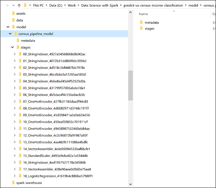
14.2 Reload the Model from the file system for use in a different context
same_pipeline_model = PipelineModel.load(MODEL_PATH)
Re-check with our best logistic regression model and this deserialized model's last stage to be same or not:
# Explains a single param and returns its name, doc, and optional default value and user-supplied value in a string.
for param in ['regParam', 'elasticNetParam', 'maxIter', 'tol']:
    same_pipeline_model.stages[-1].explainParam(param)
'regParam: regularization parameter (>= 0) (current: 0.001)'
'elasticNetParam: the ElasticNet mixing parameter, in range [0, 1]. For alpha = 0, the penalty is an L2 penalty. For alpha = 1, it is an L1 penalty (current: 1.0)'
'maxIter: maximum number of iterations (>= 0) (current: 20)'
'tol: the convergence tolerance for iterative algorithms (>= 0) (current: 1e-06)'
# Explains a single param and returns its name, doc, and optional default value and user-supplied value in a string.
for param in ['regParam', 'elasticNetParam', 'maxIter', 'tol']:
    best_log_reg_model.explainParam(param)
'regParam: regularization parameter (>= 0) (default: 0.0, current: 0.001)'
'elasticNetParam: the ElasticNet mixing parameter, in range [0, 1]. For alpha = 0, the penalty is an L2 penalty. For alpha = 1, it is an L1 penalty (default: 0.0, current: 1.0)'
'maxIter: maximum number of iterations (>= 0) (default: 100, current: 20)'
'tol: the convergence tolerance for iterative algorithms (>= 0) (default: 1e-06)'
The
'regParam',elasticNetParamand'maxIter'were provided by us and we see they are the same as the best model that resulted out of cross validation.
Generate Predictions from the deserialized model:
same_test_preds = same_pipeline_model.transform(test_df)
binary_classif_evaluator = BinaryClassificationEvaluator(labelCol="label", metricName="areaUnderROC")
areaUnderROC = binary_classif_evaluator.evaluate(same_test_preds)
print("areaUnderROC: {0}".format(areaUnderROC))
areaUnderROC: 0.904629220150728
spark.stop()
End Notes:
In this notebook, we tried to predict a person's income is above or below $50K/yr based on given features such as workclass, number of years of education, occupation, relationship, marital status, hours worked per week, race, sex etc. Seems like a simple Binary Classification task in scikit-learn and pandas; but the catch is here we did that entirely in PySpark and built a comprehensive near real-life or production grade Machine Learning worklow.
We used a Logistic Regression here. The goal of the notebook was not to get too fancy with the choice of the ML Algorithms but it was more on how can you achieve or at least try to achieve what you could do using scikit-learn and pandas. This work covered - EDA, custom udf, cleaning, basic missing values treatment, data variance per feature, stratified sampling (custom implementation), class weights for imbalanced class distribution (custom code), onehotencoding, standard scaling, vector assembling, label encoding, grid search with cross validation, pipeline, partial pipelines (custom code), binary and multi class evaluators and new metrics introduced in Spark 2.3.0, auc_roc, roc curves, model serialization and deserialization.
We also saw despite the inability to plot visualizations using Spark how can we leverage the toPandas() method to convert the aggregated DataFrames or results into Pandas DataFrame for visualization and analysis.
Going forward you can try other classification models. Also, try to convert this notebook into Scala, that would give you more exposure. In Scala, there is an UnaryTransformer class that you can use to generate the custom class-weight or logarithm of the age feature and plug that as a step into the Pipeline. In Python, its a bit tricky to do that because in order to use that we have to develop the code for the UnaryTransformer into Java or Scala first and then include that in the class path and then use that in Python.