Cell-wise analyses:reveal dominant interactions across all cells
To obtain mechanistic insights into key regulatory motifs from different perspectives, we developed three complementary strategies: cell-wise, trajectory-wise and plane-wise analyses. In this tutorial, we will introduce approaches for gene network motif analysis and guide you to perform cell-wise analyses of SPI1-GATA1 network motif.
Import relevant packages
import numpy as np
import pandas as pd
import matplotlib.pyplot as plt
# import Scribe as sb
import sys
import os
# import scanpy as sc
import dynamo as dyn
import seaborn as sns
dyn.dynamo_logger.main_silence()
adata_labeling = dyn.sample_data.hematopoiesis()
Three approaches for in-depth network motif characterizations
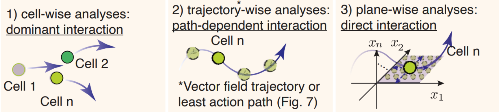
The schematic graph in this section shows the three approaches.
- cell-wise analyses to reveal dominant interactions across all cells
- trajectory-wise analyses reveal trajectory dependent interactions along a trajectory (predicted either from vector field streamline, or least action path, see Figure 6).
- Plane-wise analyses reveal direct interactions for any characteristic cell states by varying genes of interest while holding all other genes constant.
In the next section, we will use cell-wise analyses to analyze PU.1/SPI1–GATA1 network motif.
Cell-wise analyses of the PU.1/SPI1–GATA1 network motif across all cells
We showcase cell-wise analyses with the canonical PU.1/SPI1-GATA1 network motif.
Streamline plot of the RNA velocities of SPI1 (x-axis) and GATA1 (y-axis)
The streamlines of SPI1 and GATA1 show that HSPCs bifurcate into GMP-like and MEP-like branches
dyn.configuration.set_pub_style(scaler=4)
dyn.pl.streamline_plot(
adata_labeling,
color="cell_type",
x="SPI1",
y="GATA1",
layer="M_t",
ekey="M_t",
pointsize=0.5,
figsize=(8, 5),
vkey="velocity_alpha_minus_gamma_s",
)

Next we will use jacobian to show
- Repression from SPI1 to GATA1, GATA1 to SPI1
- self-activation of SPI1, and GATA1, in the SPI1 and GATA1 expression space
In particular, the repression from SPI1 to GATA1 is mostly discernable in progenitors (rectangle A: bottom left) but becomes negligible when either GATA1 is much higher than SPI1 (rectangle B: upper left) or GATA1 is close to zero (rectangle C: bottom right).
%matplotlib inline
genes = ["SPI1", "GATA1"]
def plot_jacobian_on_gene_axis(receptor, effector, x_gene=None, y_gene=None, axis_layer="M_t", temp_color_key="temp_jacobian_color", ax=None):
if x_gene is None:
x_gene = receptor
if y_gene is None:
y_gene = effector
x_axis = adata_labeling[:, x_gene].layers[axis_layer].A.flatten(),
y_axis = adata_labeling[:, y_gene].layers[axis_layer].A.flatten(),
dyn.vf.jacobian(adata_labeling, regulators = [receptor, effector], effectors=[receptor, effector])
J_df = dyn.vf.get_jacobian(
adata_labeling,
receptor,
effector,
)
color_values = np.full(adata_labeling.n_obs, fill_value=np.nan)
color_values[adata_labeling.obs["pass_basic_filter"]] = J_df.iloc[:, 0]
adata_labeling.obs[temp_color_key] = color_values
ax = dyn.pl.scatters(
adata_labeling,
vmin=0,
vmax=100,
color=temp_color_key,
cmap="bwr",
sym_c=True,
frontier=True,
sort="abs",
alpha=0.1,
pointsize=0.1,
x=x_axis,
y=y_axis,
save_show_or_return="return",
despline=True,
despline_sides=["right", "top"],
deaxis=False,
ax=ax,
)
ax.set_title(r"$\frac{\partial f_{%s}}{\partial x_{%s}}$" % (effector, receptor))
ax.set_xlabel(x_gene)
ax.set_ylabel(y_gene)
adata_labeling.obs.pop(temp_color_key)
figure, axes = plt.subplots(1, 4, figsize=(15, 3))
plot_jacobian_on_gene_axis("GATA1", "SPI1", x_gene="SPI1", y_gene="GATA1", ax=axes[0])
plot_jacobian_on_gene_axis("SPI1", "GATA1", x_gene="GATA1", y_gene="SPI1", ax=axes[1])
plot_jacobian_on_gene_axis("SPI1", "SPI1", x_gene="SPI1", y_gene="GATA1", ax=axes[2])
plot_jacobian_on_gene_axis("GATA1", "GATA1", x_gene="GATA1", y_gene="SPI1",ax=axes[3])
plt.show()
Transforming subset Jacobian: 100%|██████████| 1947/1947 [00:00<00:00, 127121.88it/s] Transforming subset Jacobian: 100%|██████████| 1947/1947 [00:00<00:00, 124848.03it/s] calculating Jacobian for each cell: 100%|██████████| 1947/1947 [00:00<00:00, 153429.97it/s] calculating Jacobian for each cell: 100%|██████████| 1947/1947 [00:00<00:00, 183195.59it/s]

The streamlines of SPI1 and GATA1 in UMAP space and colored by M_t show that HSPCs bifurcate into GMP-like and MEP-like branches clearly.
dyn.pl.streamline_plot(
adata_labeling,
color=["cell_type"],
layer="M_t",
figsize=(4, 4),
ncols=2
)
dyn.pl.streamline_plot(
adata_labeling,
color=["SPI1", "GATA1"],
layer="M_t",
figsize=(8, 4),
ncols=2
)


UMAP jacobian analysis reveals self-activation of SPI1 in GMP and GATA1 in MEP, and mutual inhibition of SPI1 and GATA1 in GMP and MEP.
dyn.vf.jacobian(adata_labeling, regulators = ["SPI1", "GATA1"])
dyn.pl.jacobian(adata_labeling, regulators = ["SPI1", "GATA1"])
Transforming subset Jacobian: 100%|██████████| 1947/1947 [00:00<00:00, 127544.78it/s]

Response heatmap
White dashed lines indicate the minimum or maximum of repression or activation and the corresponding expression threshold.
%matplotlib inline
dyn.vf.jacobian(adata_labeling, regulators=["SPI1", "GATA1"], effectors=["SPI1", "GATA1"])
dyn.pl.response(
adata_labeling,
np.array([["SPI1", "GATA1"], ["GATA1", "SPI1"], ["SPI1", "SPI1"], ["GATA1", "GATA1"]]),
ykey="jacobian",
log=False,
drop_zero_cells=True,
grid_num=25,
figsize=(5, 3),
save_show_or_return="show"
)
Transforming subset Jacobian: 100%|██████████| 1947/1947 [00:00<00:00, 125048.77it/s]

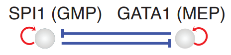
Conclusion
In the analyses above, we illustrate how to use dynamo to perform cell-wise analysis to explore the canonical PU.1/SPI1-GATA1 network motif. A schematic diagram of the SPI1-GATA1 toggle switch model can be summarized below.