Running Python code requires a running Python kernel. Click the {fa}rocket --> {guilabel}Live Code button above on this page to run the code below.

{warning}
🚧 This site is under construction! As of now, the Python kernel may not run on the page or have very long wait times. Also, expect typos.👷🏽‍♀️

(sup_class_ex)=

Example: Supervised Classification App¶

A supervised classification method fits the project requirements well and is so a good place to start. The nature of your Data and organizational needs dictate which methods you can use. So what type of data works with supervised classification methods?

One of the features (columns) contains mutually exclusive categories you want to predict (the dependent variable).
At least one other feature (the independent variable(s)).

:::{margin} Classifying non-mutually exclusive categories is called multi-label or mult-output classification. Not to be confused with multiclass classification presented in this example, multi-label classification requires different techniques, particularly with measuring accuracy. See Introduction to Multi-label Classification for more information.
:::

This will be a simple example. Simple data. Simple model. Simple interface. However, it does demonstrate the minimum requirements for part C. We'll also show how things can progressively be improved, building on the working code. Simple is a great place to start -scaling up is typically easier than going in the other direction.

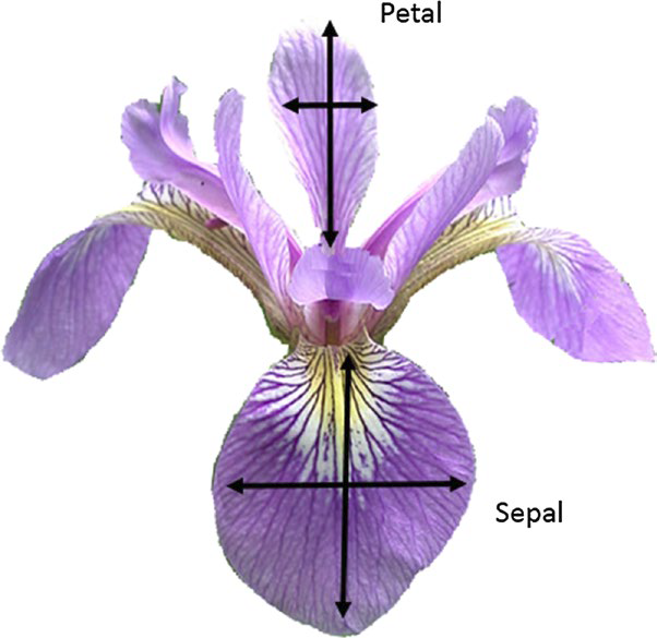
Purple iris with arrows denoting the width and length of the petal and sepal. Gird of four panels showing 2D regions defining iris type classification using independent variables sepal length and width determined by SVC using linear, linearSVC, RBF, and degree 3 polynomial kernels. The data points in each panel are divided into blue, light-blue, and red regions.

Let's look at the famous Fisher's Iris data set:

In [2]:

#We'll import libraries as needed, but when submitting, 
# it's best having them all at the top.
import pandas as pd

# Load this well-worn dataset:
url = "https://raw.githubusercontent.com/jbrownlee/Datasets/master/iris.csv"
df = pd.read_csv(url) #read CSV into Python as a DataFrame
df # displays the DataFrame

column_names = ['sepal-length', 'sepal-width', 'petal-length', 'petal-width', 'type']
df = pd.read_csv(url, names = column_names) #read CSV into Python as a DataFrame
pd.options.display.show_dimensions = False #suppresses dimension output
display(df)
#Code hide and toggle managed with Jupyter meta-code 'tags.'

	sepal-length	sepal-width	petal-length	petal-width	type
0	5.1	3.5	1.4	0.2	Iris-setosa
1	4.9	3.0	1.4	0.2	Iris-setosa
2	4.7	3.2	1.3	0.2	Iris-setosa
3	4.6	3.1	1.5	0.2	Iris-setosa
4	5.0	3.6	1.4	0.2	Iris-setosa
...	...	...	...	...	...
145	6.7	3.0	5.2	2.3	Iris-virginica
146	6.3	2.5	5.0	1.9	Iris-virginica
147	6.5	3.0	5.2	2.0	Iris-virginica
148	6.2	3.4	5.4	2.3	Iris-virginica
149	5.9	3.0	5.1	1.8	Iris-virginica

Though we described everything as "simple," we'll also see that this dataset is quite rich with angles to investigate. At this point, we have many options, but for a classification project we need a categorical feature as our dependent variable, and for this, we only have the choice: type.

In [3]:

##preserves Jupyter preview style (the '...') after applying .style. This is for presentation only. 
def display_df(dataframe, column_names, highlighted_col, precision=2):
    pd.set_option("display.precision", 2)
    columns_dict = {}
    for i in column_names:
        columns_dict[i] ='...'
    df2 = pd.concat([dataframe.iloc[:5,:],
                       pd.DataFrame(index=['...'], data=columns_dict),
                       dataframe.iloc[-5:,:]]).style.format(precision = precision).set_properties(subset=[highlighted_col], **{'background-color': 'yellow'})
    pd.options.display.show_dimensions = True
    display(df2)

#display dataframe with highlighted column 
display_df(df, column_names, 'type', 1)

	sepal-length	sepal-width	petal-length	petal-width	type
0	5.1	3.5	1.4	0.2	Iris-setosa
1	4.9	3.0	1.4	0.2	Iris-setosa
2	4.7	3.2	1.3	0.2	Iris-setosa
3	4.6	3.1	1.5	0.2	Iris-setosa
4	5.0	3.6	1.4	0.2	Iris-setosa
...	...	...	...	...	...
145	6.7	3.0	5.2	2.3	Iris-virginica
146	6.3	2.5	5.0	1.9	Iris-virginica
147	6.5	3.0	5.2	2.0	Iris-virginica
148	6.2	3.4	5.4	2.3	Iris-virginica
149	5.9	3.0	5.1	1.8	Iris-virginica

:::{sidebar} Watch

:::

The highlighted column, type provides a category to predict/classify (dependent variables), and the non-highlighted columns are something by which to make that prediction/classification (independent variables).