Notebook

An introductional notebook to HEP analysis in C++¶

In this notebook, you'll explore computing techniques commonly used in High Energy Physics (HEP) analysis. We'll guide you through creating, filling, and plotting a histogram to visualize physics data, such as the number of leptons, all in under 20 lines of code!

This tutorial also serves as an introduction to ROOT, a scientific data analysis framework. ROOT offers a comprehensive set of tools for big data processing, statistical analysis, visualization, and storage—making it useful for modern HEP research.

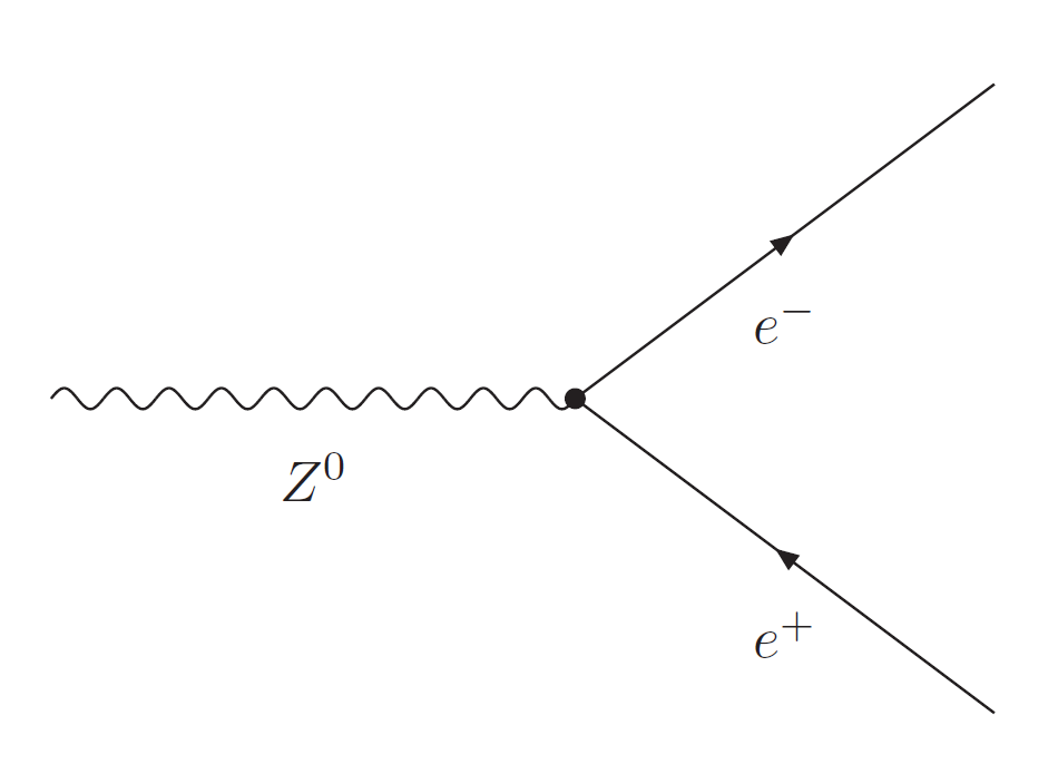
The following analysis is looking at events where Z bosons decay to two leptons of same flavour and opposite charge, (e.g., Z → e$^+$e$^-$ or Z → μ$^+$μ$^-$), as shown in the Feynman diagram.

What is the Z Boson?¶

The Z boson is one of the mediators of the weak force, which is responsible for processes such as beta decay in atomic nuclei. It interacts with all known fermions (quarks and leptons), but unlike the W boson, it does not change the type (flavor) of particle it interacts with. The Z boson couples to both left-handed and right-handed particles, making its behavior distinct from the charged W boson.

Since the Z boson is electrically neutral, its decay products must have balanced charges. The decays of the Z boson into leptons (electrons, muons, and taus) are particularly useful for experimental studies because these particles can be precisely measured in detectors, giving a clear signature of the Z boson's presence.

The Decay of the Z Boson¶

The Z boson decays rapidly due to its high mass, with a mean lifetime of around 3 × 10$^{-25}$ seconds. Its decay channels include hadrons (quarks) and leptons, but in this analysis, we are particularly interested in the lepton channels because they produce clean final states that are easier to measure.

Running a Jupyter notebook¶

A Jupyter notebook consists of cell blocks, each containing lines of Python code. Each cell can be run independently of each other, yielding respective outputs below the cells. Conventionally,cells are run in order from top to bottom.

To run the whole notebook, in the top menu click Cell $\to$ Run All.
To propagate a change you've made to a piece of code, click Cell $\to$ Run All Below.
You can also run a single code cell, by clicking Cell $\to$ Run Cells, or using the keyboard shortcut Shift+Enter.

For more information, refer to How To Use Jupyter Notebooks.

By the end of this notebook you will be able to:

Learn to process large data sets using cuts
Understand some general principles of a particle physics analysis
Discover the Z boson!

Initializing the notebook¶

To begin, we need to include several libraries that will support our analysis:

In [1]:

#include <iostream>
#include <string>
#include <stdio.h>

<iostream>: Provides input/output stream functionalities, such as printing output to the console.
<string>: Enables easy manipulation of strings.
<stdio.h>: A standard input/output library that provides functions for reading and writing data, such as printf.

To enable you interactive visualization of the histogram we'll create later, we can use the JSROOT magic command. This command activates JSROOT, a JavaScript-based ROOT viewer, allowing you to interact with the plots directly within the notebook. This makes it easier to explore the data by zooming in, rotating, or hovering over specific parts of the plot.

In [2]:

%jsroot on

Making a histogram¶

We begin by opening the data file we wish to analyze. The data is stored in a *.root* file, which consists of a tree structure containing branches and leaves. In this example, we are reading the data directly from a remote source:

In [5]:

TFile *dataFile = TFile::Open("https://atlas-opendata.web.cern.ch/atlas-opendata/samples/2020/1largeRjet1lep/MC/mc_361106.Zee.1largeRjet1lep.root");

Next, we define a tree (we'll name it *tree) to extract the data from the .root* file, from the tree called mini, that holds the data.

In [6]:

TTree *tree = (TTree*) dataFile->Get("mini");

To analyze the dataset, we need to extract specific variables. In this case, we will plot the number of leptons. Here, we bind the lep_n branch to the variable lepton_n:

In [7]:

UInt_t lepton_n = -1;
tree->SetBranchAddress("lep_n", &lepton_n);

‼️ NOTE: To know more about the contents of the ATLAS Open Data datasets, please visit our documentation.

Next, we create a canvas on which we will draw our histogram. Without a canvas, we won't be able to visualize the histogram. The following command creates a canvas named *Canvas* with a title and sets its width and height:

In [8]:

TCanvas *canvas = new TCanvas("Canvas", "A first way to plot a variable", 800, 600);

We also need to define the histogram that will be placed on this canvas. The histogram is named variable and its title is "Number of leptons". It has 5 bins that span the range from -0.5 to 4.5 (for a total range of 0 to 4 leptons):

In [9]:

TH1F *hist = new TH1F("variable","Number of leptons; Number of leptons ; Events ",5,-0.5,4.5);

The next step is to fill the histogram. We use a loop to iterate over all entries in the tree and fill the histogram for each event without applying any cuts, i.e. just copying the data as it is in the source. Once done, the word "Done!" will be printed:

In [10]:

int nentries, nbytes, i;
nentries = (Int_t)tree->GetEntries();

for (i = 0; i < nentries; i++) {
    nbytes = tree->GetEntry(i);
    hist->Fill(lepton_n);
}

std::cout << "Done!" << std::endl;

Done!

Finally, after filling the histogram, we want to visualize the results. First, we set the fill color of the histogram to red, then we draw it on the canvas, and lastly, display the canvas:

In [11]:

hist->SetFillColor(kRed);
hist->Draw();
canvas->Draw();

Interpreting the histogram¶

In the plot above, we visualize the distribution of the number of leptons per event. This histogram provides insight into the frequency of events containing different numbers of leptons.

X-axis: Represents the number of leptons detected in each event. The values range from 0 to 4, where each bin corresponds to an integer number of leptons.
Y-axis: Shows the number of events (scaled to thousands) that contain the corresponding number of leptons.

From the data:

The majority of events contain either 1 or 2 leptons, with the peak occurring at 2 leptons, suggesting that this number of leptons is the most common in the analyzed dataset.
Events with 0, 3, or 4 leptons are significantly less frequent, as indicated by the lower heights of their corresponding bins.

In the statistics box on the top right:

We see that the total number of events analyzed is 53,653.
The mean number of leptons per event is around 1.73, indicating that most events contain slightly fewer than 2 leptons on average.
The standard deviation of around 0.46 shows a relatively low spread, meaning that most events are clustered around the mean number of leptons, with little variation.

This histogram gives us a snapshot of the lepton content in the events, which can be further analyzed to study processes like lepton production in proton-proton collisions at high energies. The distribution is an important aspect of understanding the data and may inform further cuts or selection criteria for a complex physics analysis.