Kalman Filter for Bike Lean Angle Estimation
You've seen this probably on MotoGP, where the camera mounted on the bike is exactly horizontal, even when the bike leans. This is not as easy at it seems.
from IPython.display import YouTubeVideo
YouTubeVideo('-p2ndhw-kfQ', width=720, height=390)
The first try would be to use the gravitational force and just point the camera to the ground.
Doesn't work on bikes, because they are leaning in exactly this angle, which is needed to compensate the gravitational force with the centrifugal force.

One has to use two different sensors:
- a rotationrate sensor for lean angle
- a acceleration sensor for gravitional force
Both sensors have to be fused to estimate the lean angle. This is done with a Kalman Filter. We are using Sympy do develop this filter.
import numpy as np
from sympy import Symbol, symbols, Matrix, sin, cos, acos, pi
from sympy.abc import phi, g, a
from sympy import init_printing
init_printing(use_latex=True)
The state vector to describe the state of the bike consists of two variables:
$$\vec x= \left[ \matrix{ \phi \\ \dot \phi} \right]$$which is the lean angle $\phi$ (in radian) and the lean angle rate $\dot \phi$ (in radian per second).
phis = symbols('phi')
dphis = Symbol('\dot \phi')
Ts = symbols('T')
state = Matrix([phis, dphis])
state
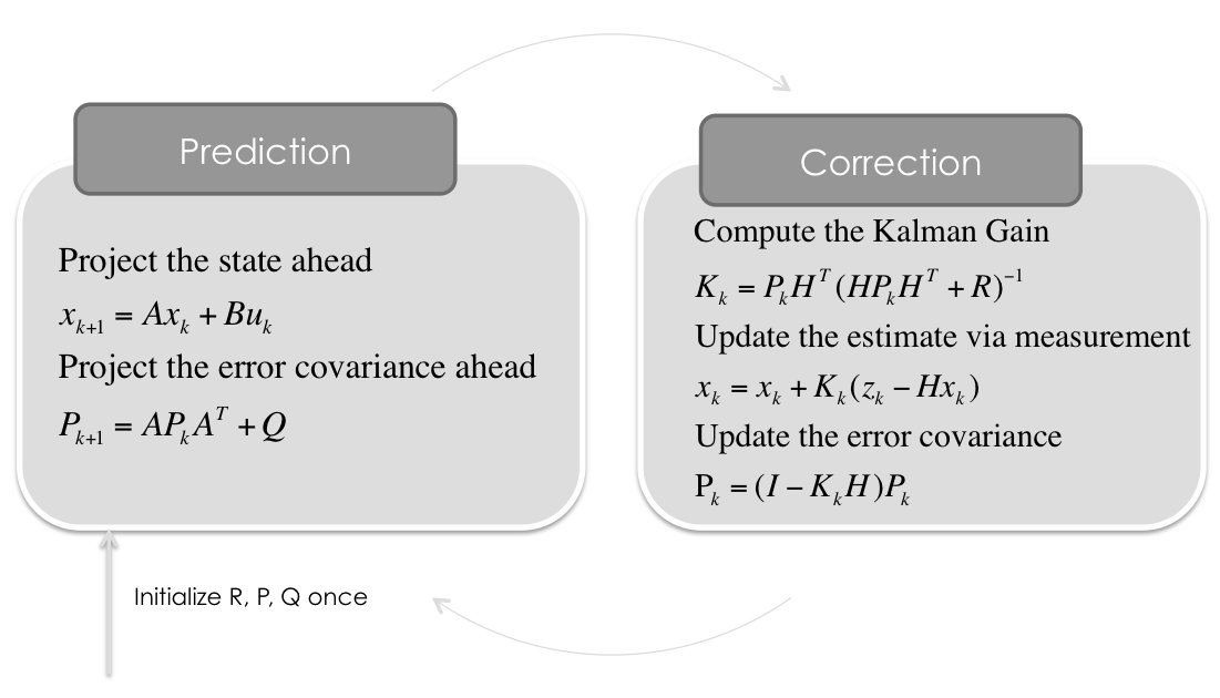
Kalman Filter Prediction Step: System Dynamics
But the state is driven by the lean angle rate $\dot \phi$ (in radian per second). So the Kalman Filter Equation for the Prediction Step is:
$$\vec x_{k+1} = A \cdot \vec x_{k}$$The dynamic matrix $A$ is simply:
$$A = \left[ \matrix{ 1 & \Delta T \\ 0 & 1 } \right]$$with $\Delta T$ as the time between two filtersteps (the sample time of the discrete Kalman Filter).
Q = np.diag([0.1, 1.0])
Kalman Filter Update Step: Sensors
We have two kind of sensors, which are usually available within a 6 Degrees of Freedom Inertial Measurement Unit (6DoF IMU):
- rotationrate sensor
- acceleration sensor
The rotationrate sensor is measuring $\dot \phi$ directly, the acceleration sensor is measuring the gravitation, so not directly the lean angle $\phi$. There is a mathematical link between the lean angle and the vertical acceleration $a$ measured by the acceleration sensor. It is the cosine. If the bike is upright, the acceleration $a$ is exactly $1g$, if it is $\phi=90^\circ$, it is $0g$.
$$a = g \cdot \cos(90^\circ - \phi)$$so the measurement function $z(x)$ is
$$\phi = 90^\circ - \arccos \left(\frac{a}{g}\right)$$a=np.linspace(-9.81, 9.81, 1000)
plt.plot(a, 90-np.arccos(a/9.81)*180.0/np.pi)
plt.xlabel('vertical Acceleration in m/s2')
plt.ylabel('lean angle in Degree')
plt.title('Lean angle as function of vertical acceleration (static!!!)')
<matplotlib.text.Text at 0x11d99e310>

Load some Measurements
%matplotlib inline
import matplotlib.pyplot as plt
import pandas as pd
data = pd.read_csv('2016-09-12-Leaning2.csv', index_col='loggingTime', parse_dates=True)
data = data[['accelerometerAccelerationX','gyroRotationY']].dropna()
dt = 1.0/50.0 # Hz
t = data.index
a_meas = data.accelerometerAccelerationX.values*-9.81 # in m/s2
a_meas[a_meas>9.81] = 9.81
a_meas[a_meas<-9.81] = -9.81
dphi_meas = data.gyroRotationY.values # in rad/s
plt.plot(np.pi/2-np.arccos(a_meas/9.81))
plt.plot(dphi_meas)
[<matplotlib.lines.Line2D at 0x11d80b310>]

Kalman Filter
x = np.matrix([[0.0],
               [0.0]]) # Initial State
A = np.matrix([[1.0, dt], [0.0, 1.0]])
H = np.diag([1.0, 1.0])
P = np.diag([100.0, 1.0])
I = np.diag([1.0, 1.0])
x0=[]
x1=[]
P0=[]
dstate=[]
for filterstep in range(len(data)):

    # Time Update (Prediction)
    # ========================
    # Project the state ahead
    x = A*x

    # Project the error covariance ahead
    P = A*P*A.T + Q


    # Measurement Update (Correction)
    # ===============================
    # Compute the Kalman Gain

    # Measurement Noise is adaptive:
    # Assuming a pretty correct angle measurement, while the
    # bike is upright (vertical acceleration is nearly 1g),
    # and a pretty bad estimation while the bike is leaning.
    # So we make the R value adaptive to the lean angle
    # with low values while upright and high values for high
    # leaning angles.
    adaptivephi = np.abs(np.multiply(1000.0,float(x[0]))+0.001)
    R = np.diag([adaptivephi, 0.001])


    S = H*P*H.T + R
    K = (P*H.T) * np.linalg.pinv(S)


    # Update the estimate via z
    Z = np.matrix([[np.pi/2-np.arccos(a_meas[filterstep]/9.81)],
                   [dphi_meas[filterstep]]])

    y = Z - (H*x)                            # Innovation or Residual
    x = x + (K*y)

    # Update the error covariance
    P = (I - (K*H))*P


    # Save states for Plotting
    x0.append(float(x[0]))
    x1.append(float(x[1]))
    P0.append(float(P[0,0]))
plt.plot(t,np.multiply(x0,180.0/np.pi), label=r'$\phi$')
#plt.plot(t,x1, label=r'$\dot \phi$')
#plt.plot(t, dphi_meas,label=r'$\dot \phi$ (ref)', alpha=0.5)
plt.title('Estimated Lean Angle')
plt.legend()
<matplotlib.legend.Legend at 0x11e01cc50>
