Bayesian Network Example with `pgmpy`, `pomegranate`, and `bnlearn`¶

Starting with pgmpy (probabilistic graphical models in python), we'll do some simple Bayesian Networks.

This demo uses the TabularCPD object to create tables of Conditional Probability Distributions (CPD). Everything should be self-explanatory and well-documented in the help, but here's some that I didn't understand at first glance:

variable_card = variable cardinality, i.e. the number of states the variable can take
evidence = list of variable names
evidence_card = cardinality of the evidence, should be a list

In pgmpy we define the network structure and the CPDs (conditional probability distributions) separately and then associate them with the structure. Here’s an example for defining the above model:

In [1]:

import pandas as pd

In [2]:

from pgmpy.models import BayesianNetwork
from pgmpy.factors.discrete import TabularCPD
from pgmpy.inference import VariableElimination

Example 1¶

This example comes from the excellent and short course by Phillip Loick on Bayesian Statistics (Udemy):

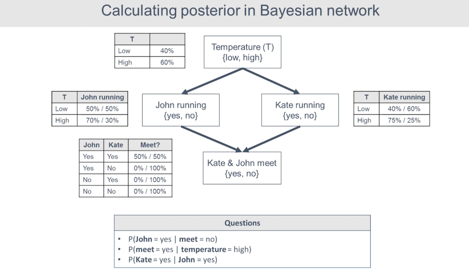
This is a fun model that models whether or not two people (John and Kate) will run based on the temperature and whether or not these two will meet.

In [3]:

# 1. Instantiate the model with node edges as a list
model = BayesianNetwork([('T', 'J'), ('T', 'K'), ('J', 'M'), ('K', 'M')])

# 2. Define the distributions
cpd_t = TabularCPD(variable='T', variable_card=2, values=[[0.4], [0.6]], state_names={'T':['low', 'high']})
cpd_j = TabularCPD(variable='J', variable_card=2, 
                   values=[[0.5, 0.7], 
                           [0.5, 0.3]], 
                   evidence=['T'],
                   evidence_card=[2],
                   state_names={'J':['yes', 'no'],
                               'T':['low', 'high']})
cpd_k = TabularCPD(variable='K', variable_card=2, 
                   values=[[0.4, 0.75], 
                           [0.6, 0.25]], 
                   evidence=['T'],
                   evidence_card=[2],
                   state_names={'K':['yes', 'no'],
                               'T':['low', 'high']})
cpd_m = TabularCPD(variable='M', variable_card = 2,
                  values=[[.5, 0, 0, 0],
                         [.5, 1, 1, 1]],
                  evidence=['J', 'K'],
                  evidence_card=[2, 2],
                  state_names={'M': ['yes', 'no'],
                              'J': ['yes', 'no'],
                              'K': ['yes', 'no']})

# 3. Add CPDs to the model
model.add_cpds(cpd_t, cpd_j, cpd_k, cpd_m)
# 4. Check the model validity (i.e. probabilities all sum to 1)
model.check_model()

Out[3]:

True

Let's doubleclick into the 'M' node because the evidence table looks different than the conditional probability table that was in the first figure:

In [4]:

# Printing a CPD with it's state names defined.
print(model.get_cpds('M'))

+--------+--------+--------+--------+-------+
| J      | J(yes) | J(yes) | J(no)  | J(no) |
+--------+--------+--------+--------+-------+
| K      | K(yes) | K(no)  | K(yes) | K(no) |
+--------+--------+--------+--------+-------+
| M(yes) | 0.5    | 0.0    | 0.0    | 0.0   |
+--------+--------+--------+--------+-------+
| M(no)  | 0.5    | 1.0    | 1.0    | 1.0   |
+--------+--------+--------+--------+-------+

This is because pgmpy expects you to have the variable states on rows and then like a multi-index of evidence on columns. Recall the evidence and evidence_card items we called out earlier as ['J', 'K'] in the TabularCPD call for variable M, so the columns show up in the order of the evidence and the state_names for each.

Inference with Variable Elimination¶

Let’s take an example of inference using Variable Elimination in pgmpy. Here we'll use our model to compute the probability distribution that the two meet, and pgmpy will make a pretty table:

In other words, what is the probability that they meet $P(M)=?$

In [5]:

from pgmpy.inference import VariableElimination

infer = VariableElimination(model)
g_dist = infer.query(['M'])
print(g_dist)

  0%|          | 0/3 [00:00<?, ?it/s]

  0%|          | 0/3 [00:00<?, ?it/s]

+--------+----------+
| M      |   phi(M) |
+========+==========+
| M(yes) |   0.1975 |
+--------+----------+
| M(no)  |   0.8025 |
+--------+----------+

You can infer conditional probabilities by adding a new term called evidence. Here we ask what's the probability that John goes for a run, given that they don't meet?

i.e.: $P(J|M=\text{no})$

In [6]:

print(infer.query(['J'], evidence={'M': 'no'}))

  0%|          | 0/2 [00:00<?, ?it/s]

  0%|          | 0/2 [00:00<?, ?it/s]

+--------+----------+
| J      |   phi(J) |
+========+==========+
| J(yes) |   0.5265 |
+--------+----------+
| J(no)  |   0.4735 |
+--------+----------+

What is $P(M=\text{yes}|T=\text{high})?$

In [7]:

print(infer.query(['M'], evidence={'T': 'high'}))

  0%|          | 0/2 [00:00<?, ?it/s]

  0%|          | 0/2 [00:00<?, ?it/s]

+--------+----------+
| M      |   phi(M) |
+========+==========+
| M(yes) |   0.2625 |
+--------+----------+
| M(no)  |   0.7375 |
+--------+----------+

What is $P(J|K)?$

In [8]:

print(infer.query(['J'], evidence={'K': 'yes'}))

  0%|          | 0/1 [00:00<?, ?it/s]

  0%|          | 0/1 [00:00<?, ?it/s]

+--------+----------+
| J      |   phi(J) |
+========+==========+
| J(yes) |   0.6475 |
+--------+----------+
| J(no)  |   0.3525 |
+--------+----------+

Example 2¶

Also from the same Udemy course, there's another example that models medical device sales and whether or not a customer is going to cancel an order.

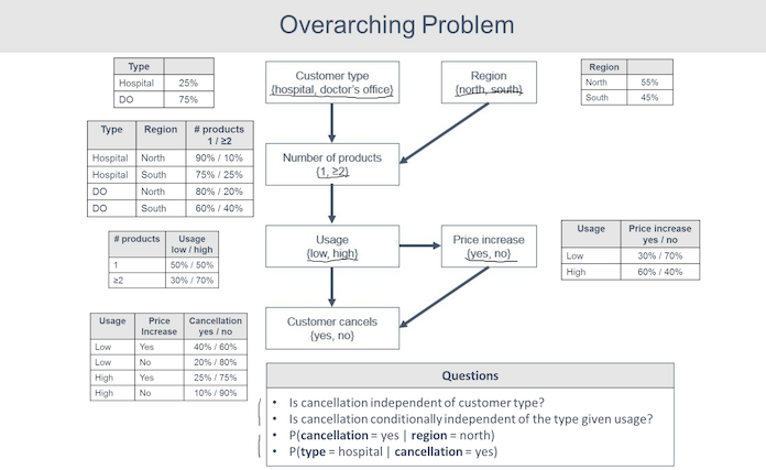
Once again, we follow the earlier pattern:

In [9]:

model = BayesianNetwork([('T', 'N'), ('R', 'N'), ('N', 'U'), ('U', 'P'), ('U', 'C'), ('P', 'C')])

T = TabularCPD(variable='T', variable_card=2, values=[[0.25], [0.75]], state_names={'T':['Hospital', 'DO']})
R = TabularCPD(variable='R', variable_card=2, values=[[0.55], [0.45]], state_names={'R':['North', 'South']})
N = TabularCPD(variable='N', variable_card=2,
                  values=[[.9, .75, .8, .6],
                         [.1, .25, .2, .4]],
                  evidence=['T', 'R'],
                  evidence_card=[2, 2],
                  state_names={'N': ['1', '≥2'],
                              'T': ['Hospital', 'DO'],
                              'R': ['North', 'South']})
U = TabularCPD(variable='U', variable_card=2,
              values=[[.5, .3],
                     [.5, .7]],
              evidence=['N'],
              evidence_card=[2],
              state_names={'U': ['low', 'high'],
                          'N': ['1', '≥2']})
P = TabularCPD(variable='P', variable_card=2,
              values=[[.3, .6],
                     [.7, .4]],
              evidence=['U'],
              evidence_card=[2],
              state_names={'P': ['yes', 'no'],
                          'U': ['low', 'high']})
C = TabularCPD(variable='C', variable_card=2,
                  values=[[.4, .2, .25, .1],
                         [.6, .8, .75, .9]],
                  evidence=['U', 'P'],
                  evidence_card=[2, 2],
                  state_names={'C': ['yes', 'no'],
                              'U': ['low', 'high'],
                              'P': ['yes', 'no']})

model.add_cpds(T, R, N, U, P, C)
model.check_model()

Out[9]:

True

In [10]:

print(model.get_cpds('C'))

+--------+--------+--------+---------+---------+
| U      | U(low) | U(low) | U(high) | U(high) |
+--------+--------+--------+---------+---------+
| P      | P(yes) | P(no)  | P(yes)  | P(no)   |
+--------+--------+--------+---------+---------+
| C(yes) | 0.4    | 0.2    | 0.25    | 0.1     |
+--------+--------+--------+---------+---------+
| C(no)  | 0.6    | 0.8    | 0.75    | 0.9     |
+--------+--------+--------+---------+---------+

Independence¶

Is customer cancellation independent of customer type?

In [11]:

# Getting all the local independencies in the network.
model.local_independencies(['C', 'T'])

Out[11]:

(C ⟂ R, T, N | P, U)
(T ⟂ R)

Type is not independent of cancellation

Next, is customer cancellation independent of customer type given usage?

Type is indeed conditionally independent of customer cancellation given usage

Inference¶

In [12]:

infer = VariableElimination(model)

Find probability that a customer cancels given that it's in the north region:

In [13]:

print(infer.query(['C'], evidence={'R': 'North'}))

  0%|          | 0/4 [00:00<?, ?it/s]

  0%|          | 0/4 [00:00<?, ?it/s]

+--------+----------+
| C      |   phi(C) |
+========+==========+
| C(yes) |   0.2226 |
+--------+----------+
| C(no)  |   0.7775 |
+--------+----------+

Find the probability that a customer is a hospital given that it is cancelled:

In [14]:

print(infer.query(['T'], evidence={'C': 'yes'}))

  0%|          | 0/4 [00:00<?, ?it/s]

  0%|          | 0/4 [00:00<?, ?it/s]

+-------------+----------+
| T           |   phi(T) |
+=============+==========+
| T(Hospital) |   0.2515 |
+-------------+----------+
| T(DO)       |   0.7485 |
+-------------+----------+

Pomegranate¶

An alternative to pgmpy is the newer pomegranate library. For bayesian networks, pomegranate offers some advantages like a built in plotting function, but interpreting the results isn't as fully developed. Furthermore, as of this writing (v 0.14.7) pomegranate can only support discrete Bayesian networks (which is fine because that's what our toy example is).

In [15]:

import pomegranate as pm

Unlike pgmpy, in pomegranate we need to specify the probabilities that John/Kate run using a DiscreteDistribution object instead of a conditional probability table. Luckily, pomegranate offers a few nice helper functions to make working with distributions faily simple:

In [16]:

# Initialize a distribution and specify parameters
T = pm.DiscreteDistribution({"low":0.4, "high":0.6})
T

Out[16]:

{
    "class" : "Distribution",
    "dtype" : "str",
    "name" : "DiscreteDistribution",
    "parameters" : [
        {
            "low" : 0.4,
            "high" : 0.6
        }
    ],
    "frozen" : false
}

We see this instantiated a Distribution object with the named parameters for each state of the discrete distribution.

pomegranate has built in plotting functions. Given this very simple distribution, we can plot the pdf with the .plot() method:

In [17]:

T.plot()

A few other useful methods:

sample(n): draw n samples from the distribution
probability(X): predict the probability of X under this distribution

In [18]:

T.sample(3)

Out[18]:

array(['low', 'high', 'high'], dtype='<U4')

In [19]:

T.probability('high')

Out[19]:

0.6

Conditional Probability Tables¶

The probability table from the first figure will need to be respecified to a 'long' format.

T	J	probability
low	yes	50%
low	no	50%
high	yes	70%
high	no	30%

The ConditionalProbabilityTable takes an argument table which is a list of lists, with each inner list is a row. A second argument parents defines the parent distributions upon which this table depends.

In [20]:

# Create the `John` variable as a conditional probability table
J = pm.ConditionalProbabilityTable(
    table=[['low', 'yes', 0.5],
           ['low', 'no', 0.5],
           ['high', 'yes', 0.7],
           ['high', 'no', 0.3]], 
    parents=[T])

So the pattern for the ConditionalProbabilityTable would look like:

parent1	variable	probability
parent1_state1	variable_state1
parent1_state1	variable_state2
etc	etc

Let's add some more nodes and build a model to examine how we can do inference.

The procedure for creating the network is as follows:

Instantiate the BayesianNetwork model
Define the distributions you want to use
Create Node objects with these distributions and add them to the model
Add edges to the model with the .add_edge(edge1, edge2) method
Bake the model using the .bake() method

In [21]:

# 1. Instantiate the BayesianNetwork model
model = pm.BayesianNetwork("Calculating Posterior")

# 2. Add more distributions
K = pm.ConditionalProbabilityTable(
    table=[['low', 'yes', 0.4],
           ['low', 'no', 0.6],
           ['high', 'yes', 0.75],
           ['high', 'no', 0.25]], parents=[T])
M = pm.ConditionalProbabilityTable(
    table=[['yes', 'yes', 'yes', 0.5],
           ['yes', 'yes', 'no', 0.5],
           ['yes', 'no', 'yes', 0],
           ['yes', 'no', 'no', 1],
           ['no', 'yes', 'yes', 0],
           ['no', 'yes', 'no', 1],
           ['no', 'no', 'yes', 0],
           ['no', 'no', 'no', 1]], parents=[J, K])

# 3. Define nodes in our network that follow these distributions
n0 = pm.Node(T, name='Temperature')
n1 = pm.Node(J, name='John')
n2 = pm.Node(K, name='Kate')
n3 = pm.Node(M, name='Meet')
model.add_states(n0, n1, n2, n3)

# 4. Define the Edges for each Node in our model
model.add_edge(n0, n1)
model.add_edge(n0, n2)
model.add_edge(n1, n3)
model.add_edge(n2, n3)

# 5. Bake the model
model.bake()

# Optional: Plot
model.plot()

I like the ability to plot (requires matplotlib and pygraphviz). Great feature!

Inference¶

We would like to do a simple inference - what's the probability that they meet?

In other words, what is the probability that they meet $P(M=\text{'yes'})$?

In pomegranate you can do this by specifying all of the probabilities like such:

In [22]:

model.probability([['high', 'yes', 'yes', 'yes'],
                  ['high', 'yes', 'no', 'yes'],
                  ['high', 'no', 'yes', 'yes'],                  
                  ['high', 'no', 'no', 'yes'],
                  ['low', 'yes', 'yes', 'yes'],
                  ['low', 'yes', 'no', 'yes'],
                  ['low', 'no', 'yes', 'yes'],                  
                  ['low', 'no', 'no', 'yes'],                   
                  ]).sum()

Out[22]:

0.19749999999999995

There is also a marginal method to get the marginal distribution of each of the variables:

In [23]:

model.marginal().shape

Out[23]:

(4,)

In [24]:

model.marginal()[3]

Out[24]:

{
    "class" : "Distribution",
    "dtype" : "str",
    "name" : "DiscreteDistribution",
    "parameters" : [
        {
            "yes" : 0.18910000000000005,
            "no" : 0.8109000000000001
        }
    ],
    "frozen" : false
}

Interesting that the marginal distribution is different than what I had calculated manually! There must be a bug in my model somewhere...

Impressions¶

It looks like it's still too early for pomegranate when it comes to Bayesian Networks when compared to pgmpy. It felt still very much WIP to use pomegranate with docstrings and help/error messages seem incomplete, while pgmpy has extensive documentation.

Classic Disease Model with `pgmpy` and `bnlearn`¶

For this next example, we'll use the classic Disease model:

Let's say that there's a disease that affects 2% of the population, and you have a 95% chance of testing positive (correctly) if you have the disease, and a 10% change of testing positive if you don't have the disease. What's the probability that you have the disease, given that you tested positive?

The Conditional Probability Table would look like:

		Test Result
		Positive	Negative
Disease	Yes	0.95	.05
Disease	No	0.90	0.1

An alternative to pgmpy is to use bnlearn which extends some of the features from pgmpy and just...does more. It can even use pgmpy objects like TabularCPD, but it looks like there are lot more convenience functions included in it to help learn from data (including the ability to handle dataframes).

In [25]:

# Import the library
import bnlearn as bn

bnlearn.make_DAG takes in an argument DAG which should be your list of edges, and a CPD argument for your conditional probability distributions that were created with pgmpy.TabularCPD.

For fun, we'll create this model with two tests ($T1$, $T2$) so we can look at statistics if you get multiple tests.

In [26]:

# Define the network structure
edges = [('D', 'T1'), ('D', 'T2')]

d = TabularCPD(variable='D', variable_card=2, values=[[0.02], [0.98]],
                  state_names={'D':['yes', 'no']})
t1 = TabularCPD(variable='T1', variable_card=2, 
                  values=[[0.95, 0.1],
                         [0.05, 0.9]],
                  evidence=['D'],
                  evidence_card=[2],
                  state_names={'D':['yes', 'no'],
                              'T1':['positive', 'negative']})
t2 = TabularCPD(variable='T2', variable_card=2, 
                  values=[[0.95, 0.1],
                         [0.05, 0.9]],
                  evidence=['D'],
                  evidence_card=[2],
                  state_names={'D':['yes', 'no'],
                              'T2':['positive', 'negative']})

# Make the actual Bayesian DAG with the previously defined CPD's 
model = bn.make_DAG(DAG=edges, CPD=[d, t1, t2])

[bnlearn] >bayes DAG created.
[bnlearn] >Add CPD: D
[bnlearn] >Add CPD: T1
[bnlearn] >Add CPD: T2
[bnlearn] >Checking CPDs..
[bnlearn] >Check for DAG structure. Correct: True

In [27]:

# Set interactive=False for web publishing
# If you have `pyviz` installed you can get an interactive graph!
bn.plot(model, title='Disease Test', interactive=False);

[bnlearn]> Set node properties.
[bnlearn]> Set edge properties.
[bnlearn] >Plot based on Bayesian model

There's also a handy print_CPD method that lets you pretty print all the CPD's.

In [28]:

bn.print_CPD(model)

CPD of D:
+--------+------+
| D(yes) | 0.02 |
+--------+------+
| D(no)  | 0.98 |
+--------+------+
CPD of T1:
+--------------+--------+-------+
| D            | D(yes) | D(no) |
+--------------+--------+-------+
| T1(positive) | 0.95   | 0.1   |
+--------------+--------+-------+
| T1(negative) | 0.05   | 0.9   |
+--------------+--------+-------+
CPD of T2:
+--------------+--------+-------+
| D            | D(yes) | D(no) |
+--------------+--------+-------+
| T2(positive) | 0.95   | 0.1   |
+--------------+--------+-------+
| T2(negative) | 0.05   | 0.9   |
+--------------+--------+-------+
[bnlearn] >Independencies:
(T2 ⟂ T1 | D)
(T1 ⟂ T2 | D)
[bnlearn] >Nodes: ['D', 'T1', 'T2']
[bnlearn] >Edges: [('D', 'T1'), ('D', 'T2')]

Inference¶

You can also use bnlearn.inference to perform inference using Variable Elimination, similar to what we saw in pgmpy:

In [29]:

bn.inference.fit(model, variables=['D'], evidence={'T1':'positive'})

[bnlearn] >Variable Elimination..

0it [00:00, ?it/s]

0it [00:00, ?it/s]

+----+-----+----------+
|    |   D |        p |
+====+=====+==========+
|  0 |   0 | 0.162393 |
+----+-----+----------+
|  1 |   1 | 0.837607 |
+----+-----+----------+

Out[29]:

<DiscreteFactor representing phi(D:2) at 0x7f91c51afaf0>

Note: Interesting that it doesn't show the 'state' names here, so the above result is 'yes' for 0 and 'no' for 1 because that's the order in which we defined the states.

Surprisingly, with the given assumptions, with a single positive test there would only be a 16% probability that you'd have the disease! What's it look like if you had two positive tests?

In [30]:

bn.inference.fit(model, variables=['D'], evidence={'T1':'positive', 'T2':'positive'})

[bnlearn] >Variable Elimination..

0it [00:00, ?it/s]

0it [00:00, ?it/s]

+----+-----+----------+
|    |   D |        p |
+====+=====+==========+
|  0 |   0 | 0.648115 |
+----+-----+----------+
|  1 |   1 | 0.351885 |
+----+-----+----------+

Out[30]:

<DiscreteFactor representing phi(D:2) at 0x7f91c51b2880>

So we see here that there's a 65% probability of having this disease after testing positive twice. A pretty dramatic improvement from the 16% earlier. But still, this is really low!

What about a real-world example with Covid testing?¶

The above example uses numbers to help surprise the learner about how counterintuitive statistics can be. But should we be skeptical of any test, especially in 2022?

If we change the prevalence and sensitivity/specificity to, say, real-world numbers for Covid-19, the numbers become more reassuring.

We can check real world numbers thanks to resources like:

Estimating disease prevalence¶

You can use the CDC Covid Tracker to get a sense of positive cases per 100K people. Let's pull the data for Multnomah County, host of the fine city of Portland, Oregon:


Source: CDC Covid Tracker

Let's say that this published rate only captures 1/4 of actual cases, due to folks not reporting (i.e. people testing at home, people who are asymptomatic and don't get tested, etc), then the true prevalence would be about 2.6%:

In [31]:

(646.86 * 4)/100000

Out[31]:

0.025874400000000002

FDA data on covid test performance¶

You can also get sensitivity and specificity data on the covid tests that the FDA approved for emergency use in the early days of the pandemic:

Here we'll use data on the Abbott AdviseDx SARS-CoV-2 IgG II (Alinity), which has a sensitivity of 98.1% (51/52), specificity of 99.6% (2000/2008). Because of the way that we've formulated this problem, we can substitute the following:

$$ \begin{aligned} \text{Sensitivity} &= P(D=\text{yes}|T=\text{'positive'}) = 51/52 = 98.0769\%\\ \text{Specificity} &= P(D=\text{no}|T=\text{'negative'}) = 2000/2008 = 99.6016\%\\ \end{aligned} $$

Or as a conditional probability table:

		Test Result
		Positive	Negative
Disease	Yes	0.981	0.019
Disease	No	0.004	0.996

For convenience, from here on out we'll redefine this as a function:

In [32]:

def disease_test(prevalence, sens, spec):
    """
    Parameters
    ----------
    prevalence : float
        Estimated percent of population that has the disease
    sens : float
        Sensitivity, or true positive rate
    spec : float
        Specificity, or true negative rate
    """
    edges = [('D', 'T1'), ('D', 'T2')]

    d = TabularCPD(variable='D', variable_card=2, values=[[prevalence], [1-prevalence]],
                      state_names={'D':['yes', 'no']})
    t1 = TabularCPD(variable='T1', variable_card=2, 
                      values=[[sens, 1-spec],
                             [1-sens, spec]],
                      evidence=['D'],
                      evidence_card=[2],
                      state_names={'D':['yes', 'no'],
                                  'T1':['positive', 'negative']})
    t2 = TabularCPD(variable='T2', variable_card=2, 
                      values=[[sens, 1-spec],
                             [1-sens, spec]],
                      evidence=['D'],
                      evidence_card=[2],
                      state_names={'D':['yes', 'no'],
                                  'T2':['positive', 'negative']})
    # Make the actual Bayesian DAG with the previously defined CPD's 
    model = bn.make_DAG(DAG=edges, CPD=[d, t1, t2], verbose=1) # quiet those messages!
    return model

In [33]:

model = disease_test(0.026, sens=51/52, spec=2000/2008)
bn.inference.fit(model, variables=['D'], evidence={'T1':'positive'})

[bnlearn] >Variable Elimination..

0it [00:00, ?it/s]

0it [00:00, ?it/s]

+----+-----+----------+
|    |   D |        p |
+====+=====+==========+
|  0 |   0 | 0.867923 |
+----+-----+----------+
|  1 |   1 | 0.132077 |
+----+-----+----------+

Out[33]:

<DiscreteFactor representing phi(D:2) at 0x7f91c54f2be0>

Reassuringly, the probability of having the disease is about 87%, after having tested positive with this test (and assuming prevalence of 2.6%).

In [34]:

bn.inference.fit(model, variables=['D'], evidence={'T1':'positive', 'T2':'positive'})

[bnlearn] >Variable Elimination..

0it [00:00, ?it/s]

0it [00:00, ?it/s]

+----+-----+-------------+
|    |   D |           p |
+====+=====+=============+
|  0 |   0 | 0.999382    |
+----+-----+-------------+
|  1 |   1 | 0.000617783 |
+----+-----+-------------+

Out[34]:

<DiscreteFactor representing phi(D:2) at 0x7f91c54e0640>

And after 2 tests, the probability rises to 99.9%. Not bad, right?

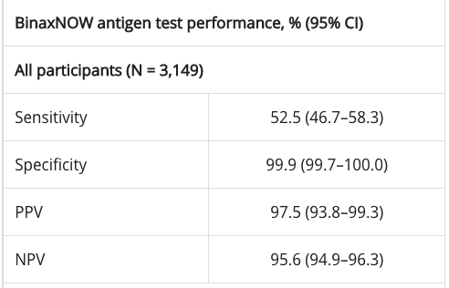
Now, let's take a quick look with a rapid at-home test like the Abbot BinaxNOW test. There seems to be some conflicting data on this (i.e. the results are better if you're symptomatic), but we can try to use some available overall numbers. Skimming the results of Table 2 from this Nov 2020 study gives us a Sensitivity of 52.5% and Specificity of 99.9%:



From: Prince-Guerra JL, Almendares O, Nolen LD, et al. Evaluation of Abbott BinaxNOW Rapid Antigen Test for SARS-CoV-2 Infection at Two Community-Based Testing Sites — Pima County, Arizona, November 3–17, 2020. MMWR Morb Mortal Wkly Rep 2021

In [35]:

model = disease_test(0.026, sens=0.525, spec=0.999)
bn.inference.fit(model, variables=['D'], evidence={'T1':'positive'})

[bnlearn] >Variable Elimination..

0it [00:00, ?it/s]

0it [00:00, ?it/s]

+----+-----+-----------+
|    |   D |         p |
+====+=====+===========+
|  0 |   0 | 0.933397  |
+----+-----+-----------+
|  1 |   1 | 0.0666028 |
+----+-----+-----------+

Out[35]:

<DiscreteFactor representing phi(D:2) at 0x7f91c5515610>

So that's quite good, considering the study found that sensitivity was much higher among symptomatic patients. We can also take a look if you take two tests:

In [36]:

bn.inference.fit(model, variables=['D'], evidence={'T1':'positive', 'T2':'positive'})

[bnlearn] >Variable Elimination..

0it [00:00, ?it/s]

0it [00:00, ?it/s]

+----+-----+-------------+
|    |   D |           p |
+====+=====+=============+
|  0 |   0 | 0.999864    |
+----+-----+-------------+
|  1 |   1 | 0.000135896 |
+----+-----+-------------+

Out[36]:

<DiscreteFactor representing phi(D:2) at 0x7f91c554aac0>

And now there's near certainty with two tests. What if you had one test positive and another negative, out of curiosity?

In [37]:

bn.inference.fit(model, variables=['D'], evidence={'T1':'positive', 'T2':'negative'})

[bnlearn] >Variable Elimination..

0it [00:00, ?it/s]

0it [00:00, ?it/s]

+----+-----+----------+
|    |   D |        p |
+====+=====+==========+
|  0 |   0 | 0.869511 |
+----+-----+----------+
|  1 |   1 | 0.130489 |
+----+-----+----------+

Out[37]:

<DiscreteFactor representing phi(D:2) at 0x7f91c5563760>

References¶

In [ ]:

Bayesian Network Example with pgmpy, pomegranate, and bnlearn¶

Example 1¶

Inference with Variable Elimination¶

Example 2¶

Independence¶

Inference¶

Pomegranate¶

Conditional Probability Tables¶

Inference¶

Impressions¶

Classic Disease Model with pgmpy and bnlearn¶

Inference¶

What about a real-world example with Covid testing?¶

Estimating disease prevalence¶

FDA data on covid test performance¶

References¶

Bayesian Network Example with `pgmpy`, `pomegranate`, and `bnlearn`¶

Classic Disease Model with `pgmpy` and `bnlearn`¶