Silver nanoparticle response to Bovine Serum Albumina (BSA)
In section 03_LSPR_sensor_response_POC of this report we present a proof of concept of Localized surface plasmon resonance sensor (LSPR) response. We show how PyGBe can be used to model the response of LSPR biosensors by modeling the BSA as spheres.
In this report, we present a more realistic approach where we use the geometry of the actual protein and its charges. We obtain the crystal structure of BSA (4f5s) from the Protein Data Bank and generate the charge distibution and mesh using pdb2pqr and NanoShaper respectively.
We study the interaction between a realistic model of the BSA protein (non-spherical) and the nanoparticle; more specifically how the relative position between them affects sensitivity.

#### Fig 1. Setup for response calculation using crystal structure of real protein.
Mesh convergence
Before running the response calculations we perform a mesh convergence analysis to ensure that the results are not going to be affected by changing the size of the mesh.
Since we compute the extinction cross section over the sphere nanoparticle, we pick a fixed mesh density for the protein and varied the refinement over the sphere. After studying different cases we decide to use a mesh of density 2 triangles per Angstrom square for the protein.
We run the case presented in Fig. 1 for radius of the sphere of $25 \, nm$, a wavelength of $380 \, nm$ and a distance $d\,=\,1 \,nm$ for meshes of 512, 2048, 8192 and 32768 elements.
The values for the dielectric constants for water and silver were obtained by interpolation of experimental data (2,3):
- Water : 1.7972 + 8.5048e-09j
- Silver: -3.3877 + 0.1922j
For the protein (modeled as a sphere) we use Bovine Serum Albumina (BSA) data extracted from the functional relationship provided by Pahn, et al. (1)
- Protein: 2.7514 + 0.2860j
The parameters used to perform the convergence analysis are:
Precision   double
K           4
Nk          9
K_fine      37
thresold    0.5
BSZ         128
restart     100
tolerance   1e-5
max_iter    1000
P           15
eps         1e-12
NCRIT       500
theta       0.5
GPU         1
The error calculation uses the Richardson extrapolation value of the extinction cross-section as a reference, $Cext\,=\, 6799.27 \, nm^2$. We obtain an order of convergence of $0.98$
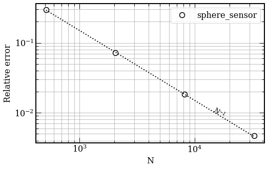
#### Fig 2. Convergence of extinction cross-section of a $r=25\, nm$ silver sphere with BSA protein located at $1\,nm$ away along the z-axis, versus the number of elements.
Relaxiation of parameters to optimize run time
We analyzed different combinations of simulation parameters in order to reduce the time of computation and have a relative error (compared to the Richardson extrapolation) smaller %2.
The final parameters picked are:
Density of protein mesh: 1 triangle/Ang^2
Precision   double
K           4
Nk          9
K_fine      19
thresold    0.5
BSZ         128
restart     100
tolerance   1e-3
max_iter    1000
P           6
eps         1e-12
NCRIT       500
theta       0.5
GPU         1
After this relaxation the percentage error compared to the Richardson extrapolation is %0.63 and the time of computation is approximately 7.5 min in a K40.
References
(1) Phan, Anh D., et al. "Surface plasmon resonances of protein-conjugated gold nanoparticles on graphitic substrates." Applied Physics Letters 103.16 (2013): 163702.
(2) Hale, G. M. and Querry, M. R. (1972). Optical constants of water in the 200-nm to 200-μm wavelength region. Appl. Opt., 12(3):555–563.
(3) Johnson, P. B. and Christy, R. W. (1972). Optical constants of nobble metals. Phys. Rev. B, 12(6):4370–4379.
#Ignore this cell, It simply loads a style for the notebook.

from IPython.core.display import HTML
def css_styling():
    try:
        styles = open("styles/custom.css", "r").read()
        return HTML(styles)
    except:
        pass
css_styling()