Notebook

Regression¶

Preliminaries¶

Goal
- Introduction to Bayesian (Linear) Regression
Materials
- Mandatory
  - These lecture notes
- Optional
  - Bishop pp. 152-158
  - In this and forthcoming lectures, we will make use of some elementary matrix calculus. The most important formulas are summarized at the bottom of this notebook in an OPTIONAL SLIDE on matrix calculus. For derivations, see Bishop Appendix C.

Regression - Illustration¶

Given a set of (noisy) data measurements, find the 'best' relation between an input variable $x \in \mathbb{R}^M$ and input-dependent outcomes $y \in \mathbb{R}$.

Regression vs Density Estimation¶

Observe $N$ IID data pairs $D=\{(x_1,y_1),\dotsc,(x_N,y_N)\}$ with $x_n \in \mathbb{R}^M$ and $y_n \in \mathbb{R}$.

Assume that we are interested in (a model for) the responses $y_n$ for given inputs $x_n$?, I.o.w. we are interested in building a model for the conditional distribution $p(y|x)$.

Note that, since $p(x,y)=p(y|x)\, p(x)$, building a model $p(y|x)$ is similar to density estimation with the assumption that $x$ is drawn from a uniform distribution.

Bayesian Linear Regression¶

Next, we discuss (1) model specification, (2) Inference and (3) a prediction application for a Bayesian linear regression problem.

1. Model Specification¶

In a traditional regression model, we try to 'explain the data' by a purely deterministic function $f(x_n,w)$, plus a purely random term $\epsilon_n$ for 'unexplained noise':

$$ y_n = f(x_n,w) + \epsilon_n $$

In a linear regression model, i.e., linear w.r.t. the parameters $w$, we assume that

$$f(x_n,w)= \sum_{j=0}^{M-1} w_j \phi_j(x_n) = w^T \phi(x_n)$$

where $\phi_j(x)$ are called basis functions.

For notational simplicity, from now on we will assume $f(x_n,w) = w^T x_n$, with $x_n \in \mathbb{R}^M$.

In ordinary linear regression , the noise process $\epsilon_n$ is zero-mean Gaussian with constant variance, i.e.

$$ \epsilon_n \sim \mathcal{N}(0,\beta^{-1}) \,. $$

Hence, given a data set $D=\{(x_1,y_1),\dotsc,(x_N,y_N)\}$, the likelihood for an ordinary linear regression model is

$$\begin{align*} p(y\,|\,\mathbf{X},w,\beta) &= \mathcal{N}(y\,|\,\mathbf{X} w,\beta^{-1} \mathbf{I}) \\ &= \prod_n \mathcal{N}(y_n\,|\,w^T x_n,\beta^{-1}) \tag{B-3.10} \end{align*}$$

where $w = \left(\begin{matrix} w_1 \\ w_2 \\ \vdots \\ w_{M} \end{matrix} \right)$, the $(N\times M)$-dim matrix $\mathbf{X} = \left(\begin{matrix}x_1^T \\ x_2^T \\ \vdots \\ x_N^T \end{matrix} \right) = \left(\begin{matrix}x_{11},x_{12},\dots,x_{1M}\\ x_{21},x_{22},\dots,x_{2M} \\ \vdots \\ x_{N1},x_{N2},\dots,x_{NM} \end{matrix} \right) $ and $y = \left(\begin{matrix} y_1 \\ y_2 \\ \vdots \\ y_N \end{matrix} \right)$.

For full Bayesian learning we should also choose a prior $p(w)$:

$$\begin{equation} p(w\,|\,\alpha) = \mathcal{N}(w\,|\,0,\alpha^{-1}\mathbf{I}) \tag{B-3.52} \end{equation}$$

For simplicity, we will assume that $\alpha$ and $\beta$ are fixed and known.

2. Inference¶

We'll do Bayesian inference for the parameters $w$.

$$\begin{align*} p(w|D) &\propto p(D|w)\cdot p(w) \\ &= \mathcal{N}(y\,|\,\mathbf{X} w,\beta^{-1} \mathbf{I}) \cdot \mathcal{N}(w\,|\,0,\alpha^{-1}\mathbf{I}) \\ &\propto \exp \big( -\frac{\beta}{2} \big( {y - \mathbf{X}w } \big)^T \big( {y - \mathbf{X}w } \big) - \frac{\alpha}{2}w^T w \big) \qquad \text{(B-3.55)} \\ &= \exp\big( -\frac{1}{2} w^T\big(\underbrace{\beta \mathbf{X}^T\mathbf{X} + \alpha \mathbf{I}}_{\Lambda_N}\big)w + \big(\underbrace{\beta \mathbf{X}^Ty}_{\eta_N}\big)^T w - \frac{\beta}{2}y^T y \big) \\ &\propto \mathcal{N}_c\left(w\,|\,\eta_N,\Lambda_N \right) \end{align*}$$

with natural parameters (see the natural parameterization of Gaussian):

$$\begin{align*} \eta_N &= \beta\mathbf{X}^Ty \\ \Lambda_N &= \beta \mathbf{X}^T\mathbf{X} + \alpha \mathbf{I} \end{align*}$$

Or equivalently (in the moment parameterization of the Gaussian):

$$\begin{align*} p(w|D) &= \mathcal{N}\left(w\,|\,m_N,S_N \right) \qquad &&\text{(B-3.49)} \\ m_N &= \beta S_N \mathbf{X}^T y \qquad &&\text{(B-3.53)}\\ S_N &= \left(\alpha \mathbf{I} + \beta \mathbf{X}^T \mathbf{X}\right)^{-1} \qquad &&\text{(B-3.54)} \end{align*}$$

Note that B-3.53 and B-3.54 combine to

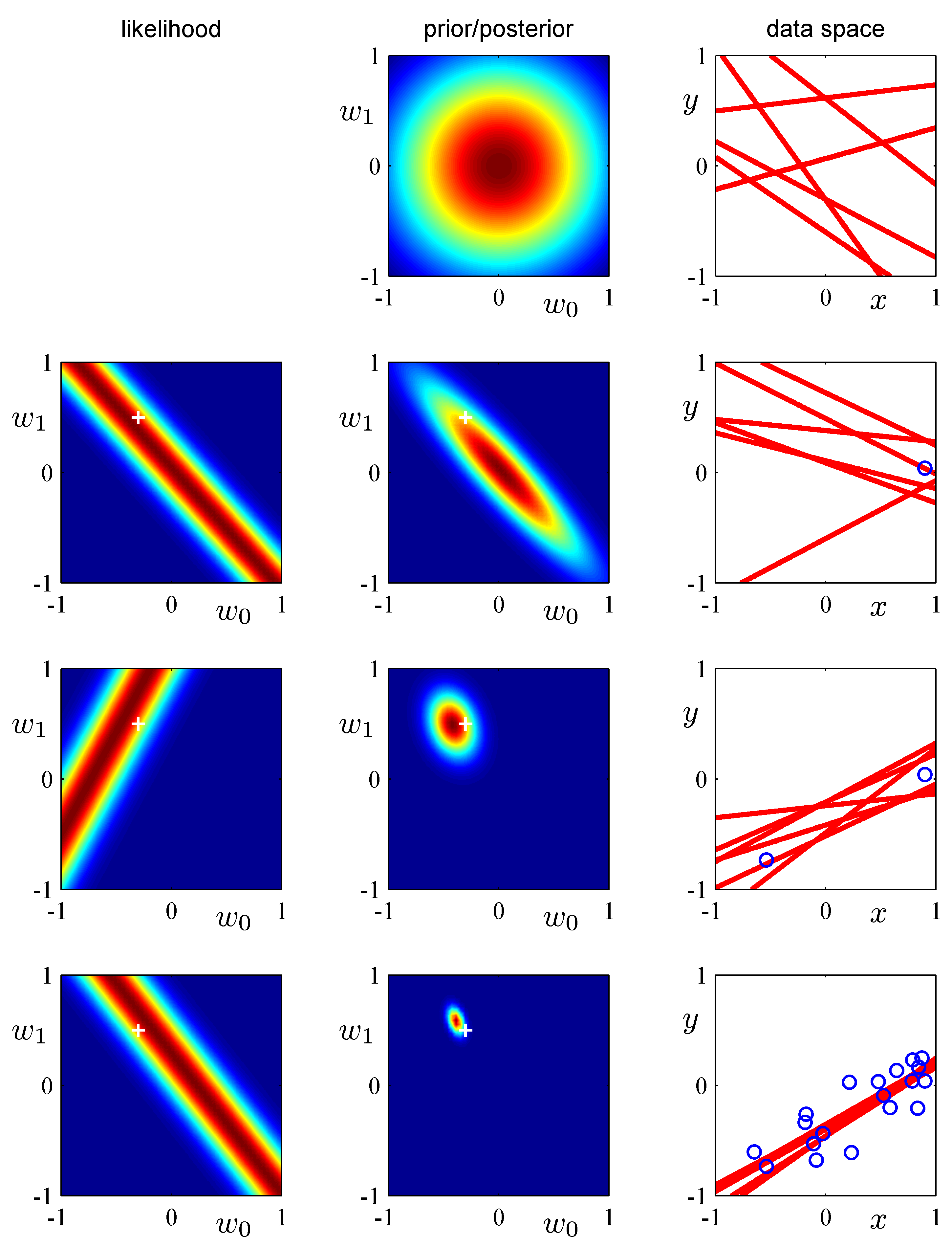
$$ m_N = \left(\frac{\alpha}{\beta}\mathbf{I} + \mathbf{X}^T \mathbf{X} \right)^{-1} \mathbf{X}^T y\,. $$

(Bishop Fig.3.7) Illustration of sequential Bayesian learning for a simple linear model of the form $y(x, w) =

w_0 + w_1 x$. (Bishop Fig.3.7, detailed description at Bishop, pg.154.)

3. Application: Predictive Distribution ¶

Assume we are interested in the distribution $p(y_\bullet \,|\, x_\bullet, D)$ for a new input $x_\bullet$. This can be worked out as (exercise B-3.10)

$$\begin{align*} p(y_\bullet \,|\, x_\bullet, D) &= \int p(y_\bullet \,|\, x_\bullet, w) p(w\,|\,D)\,\mathrm{d}w \\ &= \int \mathcal{N}(y_\bullet \,|\, w^T x_\bullet, \beta^{-1}) \mathcal{N}(w\,|\,m_N,S_N)\,\mathrm{d}w \\ &= \int \mathcal{N}(y_\bullet \,|\, z, \beta^{-1}) \underbrace{\mathcal{N}(z\,|\,x_\bullet^T m_N,x_\bullet^T S_N x_\bullet)\,\mathrm{d}z}_{=\mathcal{N}(w\,|\,m_N,S_N)\,\mathrm{d}w} \quad \text{(sub. }z=x_\bullet^T w \text{)} \\ &= \int \underbrace{\underbrace{\mathcal{N}(z \,|\, y_\bullet, \beta^{-1})}_{\text{switch }z \text{ and }y_\bullet} \mathcal{N}(z\,|\,x_\bullet^T m_N,x_\bullet^T S_N x_\bullet)}_{\text{Use Gaussian product formula SRG-6}}\,\mathrm{d}z \\ &= \int \mathcal{N}\left(y_\bullet\,|\, m_N^T x_\bullet, \sigma_N^2(x_\bullet) \right) \underbrace{\mathcal{N}\left(z\,|\, \cdot, \cdot\right)}_{\text{integrate this out}} \mathrm{d}z\\ &= \mathcal{N}\left(y_\bullet\,|\, m_N^T x_\bullet, \sigma_N^2(x_\bullet) \right) \end{align*}$$

with $$\begin{align*} \sigma_N^2(x_\bullet) = \beta^{-1} + x^T_\bullet S_N x_\bullet \tag{B-3.59} \end{align*}$$

So, the uncertainty $\sigma_N^2(x_\bullet)$ about the output $y_\bullet$ contains both uncertainty about the process ($\beta^{-1}$) and about the model parameters ($x^T_\bullet S_N x_\bullet$).
(See the OPTIONAL SLIDE below for the step in this derivation where $\mathcal{N}(w\,|\,m_N,S_N)\,\mathrm{d}w$ gets replaced $\mathcal{N}(z\,|\,x_\bullet^T m_N,x_\bullet^T S_N x_\bullet)\,\mathrm{d}z$.)

Example Predictive Distribution¶

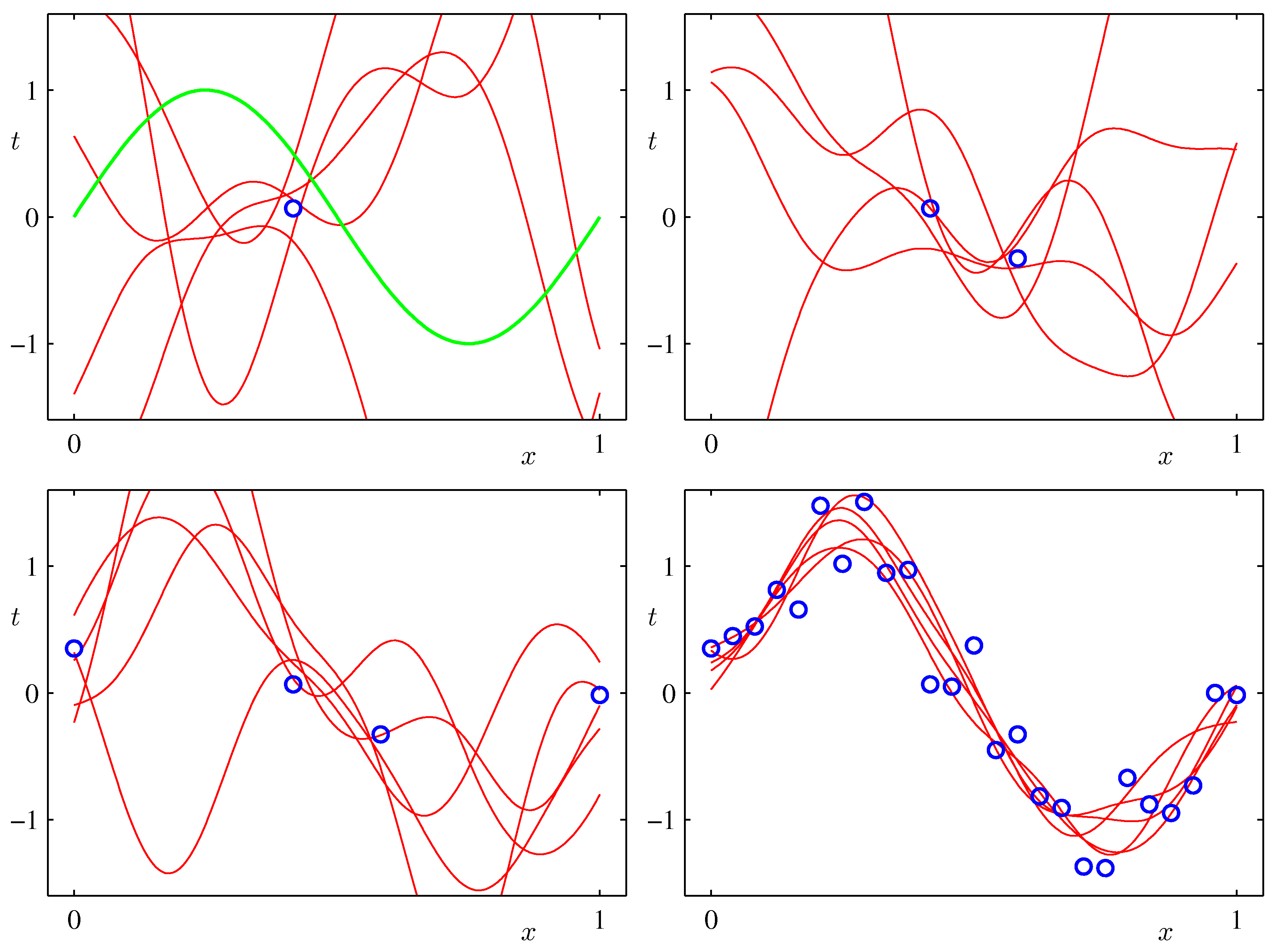
As an example, let's do Bayesian Linear Regression for a synthetic sinusoidal data set and a model with 9 Gaussian basis functions

$$\begin{align*} y_n &=\sum_{m=1}^9 w_m \phi_m(x_n) + \epsilon_n \\ \phi_m(x_n) &= \exp\left( \frac{x_n-\mu_m}{\sigma^2}\right) \\ \epsilon_n &\sim \mathcal{N}(0,\beta^{-1}) \end{align*}$$

The predictive distributions for $y$ are shown in the following plots (Bishop, Fig.3.8)

And some plots of draws of posteriors for the functions $w^T \phi(x)$ (Bishop, Fig.3.9)

Maximum Likelihood Estimation for Linear Regression Model¶

Recall the posterior mean for the weight vector

$$ m_N = \left(\frac{\alpha}{\beta}\mathbf{I} + \mathbf{X}^T \mathbf{X} \right)^{-1} \mathbf{X}^T y $$

where $\alpha$ is the prior precision for the weights.

The Maximum Likelihood solution for $w$ is obtained by letting $\alpha \rightarrow 0$, which leads to

$$\begin{equation*} \hat w_{\text{ML}} = (\mathbf{X}^T \mathbf{X})^{-1} \mathbf{X}^T y \end{equation*}$$

The matrix $\mathbf{X}^\dagger \equiv (\mathbf{X}^T \mathbf{X})^{-1}\mathbf{X}^T$ is also known as the Moore-Penrose pseudo-inverse (which is sort-of-an-inverse for non-square matrices).

Note that if we have fewer training samples than input dimensions, i.e., if $N<M$, then $\mathbf{X}^T \mathbf{X}$ will not be invertible and maximum likelihood blows up. The Bayesian solution does not suffer from this problem.

Least-Squares Regression¶

(You may say that) we don't need to work with probabilistic models. E.g., there's also the deterministic least-squares solution: minimize sum of squared errors,

$$\begin{align*} \hat w_{\text{LS}} &= \arg\min_{w} \sum_n {\left( {y_n - w ^T x_n } \right)} ^2 = \arg\min_{w} \left( {y - \mathbf{X}w } \right)^T \left( {y - \mathbf{X} w } \right) \end{align*}$$

Setting the gradient

$ \frac{\partial \left( {y - \mathbf{X}w } \right)^T \left( {y - \mathbf{X}w } \right)}{\partial w} = -2 \mathbf{X}^T \left(y - \mathbf{X} w \right) $ to zero yields the so-called normal equations $\mathbf{X}^T\mathbf{X} \hat w_{\text{LS}} = \mathbf{X}^T y$ and consequently

$$ \hat w_{\text{LS}} = (\mathbf{X}^T \mathbf{X})^{-1} \mathbf{X}^T y $$

which is the same answer as we got for the maximum likelihood weights $\hat w_{\text{ML}}$.

$\Rightarrow$ Least-squares regression ($\hat w_{\text{LS}}$) corresponds to the (probabilistic) maximum likelihood solution ($\hat w_{\text{ML}}$) if the probabilistic model includes the following assumptions:
1. The observations are independently and identically distributed (IID) (this determines how errors are combined), and
2. The noise signal $\epsilon_n \sim \mathcal{N}(0,\,\beta^{-1})$ is Gaussian distributed (determines the error metric)

If you use the Least-Squares method, you cannot see (nor modify) these assumptions. The probabilistic method forces you to state all assumptions explicitly!

Not Identically Distributed Data¶

Let's do an example regarding changing our assumptions. What if we assume that the variance of the measurement error varies with the sampling index, $\epsilon_n \sim \mathcal{N}(0,\beta_n^{-1})$?

The likelihood is now (using $\Lambda \triangleq \mathrm{diag}(\beta_n)$ )

$$ p(y\,|\,\mathbf{X},w,\Lambda) = \mathcal{N}(y\,|\,\mathbf{X} w,\Lambda^{-1} ) \,. $$

Combining this likelihood with the prior $p(w) = \mathcal{N}(w\,|\,0,\alpha^{-1}\mathbf{I})$ leads to a posterior

$$\begin{align*} p(w|D) &\propto p(D|w)\cdot p(w) \\ &= \mathcal{N}(y\,|\,\mathbf{X} w,\Lambda^{-1} \mathbf{I}) \cdot \mathcal{N}(w\,|\,0,\alpha^{-1}\mathbf{I}) \\ &\propto \exp \left\{ \frac{1}{2} \left( {y - \mathbf{X}w } \right)^T \Lambda \left( {y - \mathbf{X}w } \right) + \frac{\alpha}{2}w^T w \right\} \\ &\propto \mathcal{N}\left(w\,|\,m_N,S_N \right) \end{align*}$$

with $$\begin{align*} m_N &= S_N \mathbf{X}^T \Lambda y \\ S_N &= \left(\alpha \mathbf{I} + \mathbf{X}^T \Lambda \mathbf{X}\right)^{-1} \end{align*}$$

And maximum likelihood solution

$$ \hat{w}_{\text{ML}} = \left. m_N\right|_{\alpha \rightarrow 0} = \left(\mathbf{X}^T \Lambda \mathbf{X}\right)^{-1} \mathbf{X}^T \Lambda y $$

This maximum likelihood solution is also called the Weighted Least Squares (WLS) solution. (Note that we just stumbled upon it, the crucial aspect is appropriate model specification!)

Note also that the dimension of $\Lambda$ grows with the number of data points. In general, models for which the number of parameters grow as the number of observations increase are called non-parametric models.

Code Example: Least Squares vs Weighted Least Squares¶

We'll compare the Least Squares and Weighted Least Squares solutions for a simple linear regression model with input-dependent noise:

$$\begin{align*} x &\sim \text{Unif}[0,1]\\ y|x &\sim \mathcal{N}(f(x), v(x))\\ f(x) &= 5x - 2\\ v(x) &= 10e^{2x^2}-9.5\\ \mathcal{D} &= \{(x_1,y_1),\ldots,(x_N,y_N)\} \end{align*}$$

In [1]:

using PyPlot, LinearAlgebra

# Model specification: y|x ~ 𝒩(f(x), v(x))
f(x) = 5*x .- 2 
v(x) = 10*exp.(2*x.^2) .- 9.5 # input dependent noise variance
x_test = [0.0, 1.0]
plot(x_test, f(x_test), "k--") # plot f(x)

# Generate N samples (x,y), where x ~ Unif[0,1]
N = 50
x = rand(N)
y = f(x) + sqrt.(v(x)) .* randn(N)
plot(x, y, "kx"); xlabel("x"); ylabel("y") # Plot samples

# Add constant to input so we can estimate both the offset and the slope
_x = [x ones(N)]
_x_test = hcat(x_test, ones(2))

# LS regression
w_ls = pinv(_x) * y
plot(x_test, _x_test*w_ls, "b-") # plot LS solution

# Weighted LS regression
W = Diagonal(1 ./ v(x)) # weight matrix
w_wls = inv(_x'*W*_x) * _x' * W * y
plot(x_test, _x_test*w_wls, "r-") # plot WLS solution
ylim([-5,8]); legend(["f(x)", "D", "LS linear regr.", "WLS linear regr."],loc=2);

OPTIONAL SLIDES¶

Some Useful Matrix Calculus ¶

When doing derivatives with matrices, e.g. for maximum likelihood estimation, it will be helpful to be familiar with some matrix calculus. We shortly recapitulate used formulas here.

We define the gradient of a scalar function $f(A)$ w.r.t. an $n \times k$ matrix $A$ as

$$ \nabla_A f \triangleq \begin{bmatrix} \frac{\partial{f}}{\partial a_{11}} & \frac{\partial{f}}{\partial a_{12}} & \cdots & \frac{\partial{f}}{\partial a_{1k}}\\ \frac{\partial{f}}{\partial a_{21}} & \frac{\partial{f}}{\partial a_{22}} & \cdots & \frac{\partial{f}}{\partial a_{2k}}\\ \vdots & \vdots & \cdots & \vdots\\ \frac{\partial{f}}{\partial a_{n1}} & \frac{\partial{f}}{\partial a_{n2}} & \cdots & \frac{\partial{f}}{\partial a_{nk}} \end{bmatrix} $$

The following formulas are useful (see Bishop App.-C)

$$\begin{align*} |A^{-1}|&=|A|^{-1} \tag{B-C.4} \\ \nabla_A \log |A| &= (A^{T})^{-1} = (A^{-1})^T \tag{B-C.28} \\ \mathrm{Tr}[ABC]&= \mathrm{Tr}[CAB] = \mathrm{Tr}[BCA] \tag{B-C.9} \\ \nabla_A \mathrm{Tr}[AB] &=\nabla_A \mathrm{Tr}[BA]= B^T \tag{B-C.25} \\ \nabla_A \mathrm{Tr}[ABA^T] &= A(B+B^T) \tag{B-C.27}\\ \nabla_x x^TAx &= (A+A^T)x \tag{from B-C.27}\\ \nabla_X a^TXb &= \nabla_X \mathrm{Tr}[ba^TX] = ab^T \notag \end{align*}$$

Derivation Predictive Distribution ¶

In the derivation of the predictive distribution, we replaced $\mathcal{N}(w\,|\,m_N,S_N)\,\mathrm{d}w$ with $\mathcal{N}(z\,|\,x_\bullet^T m_N,x_\bullet^T S_N x_\bullet)\,\mathrm{d}z$. Here we discuss why that is allowed.
Since $z = x^T w$ (drop the bullet for notational simplicity), we have

$$p(z) = \mathcal{N}(z|m_z,S_z)$$

with $$\begin{aligned} m_z &:= E[z] = E[x^T w] = x^T E[w] = x^T m_N \\ \Sigma_z &:= E[(z-m_z)(z-m_z)^T] \\ &= E[(x^T w - x^T m_N)(x^T w - x^T m_N)^T] \\ &= x^T E[(w - m_N)(w - m_N)^T]x \\ &= x^T S_N x \end{aligned}$$

Then we equate probability masses in both domains:

$$ \mathcal{N}(z|m_z,\Sigma_z)\mathrm{d}z = \mathcal{N}(w|m_N,S_N)\mathrm{d}w$$$$ \Rightarrow \mathcal{N}(z|x^T m_N,x^T S_N x)\mathrm{d}z = \mathcal{N}(w|m_N,S_N)\mathrm{d}w $$