Notebook

Factor Graphs¶

Preliminaries¶

Goal
- Introduction to Forney-style factor graphs and message passing-based inference
Materials
- Mandatory
  - These lecture notes
  - Loeliger (2007), The factor graph approach to model based signal processing, pp. 1295-1302 (until section V)
- Optional
  - Frederico Wadehn (2015), Probabilistic graphical models: Factor graphs and more video lecture (recommended)
- References
  - Forney (2001), Codes on graphs: normal realizations

Why Factor Graphs?¶

A probabilistic inference task gets its computational load mainly through the need for marginalization (i.e., computing integrals). E.g., for a model $p(x_1,x_2,x_3,x_4,x_5)$, the inference task $p(x_2|x_3)$ is given by

$$ p(x_2|x_3) = \frac{p(x_2,x_3)}{p(x_3)} = \frac{\int \cdots \int p(x_1,x_2,x_3,x_4,x_5) \, \mathrm{d}x_1 \mathrm{d}x_4 \mathrm{d}x_5}{\int \cdots \int p(x_1,x_2,x_3,x_4,x_5) \, \mathrm{d}x_1 \mathrm{d}x_2 \mathrm{d}x_4 \mathrm{d}x_5}$$

Since these computations (integrals or sums) suffer from the "curse of dimensionality", we often need to solve a simpler problem in order to get an answer.

Factor graphs provide a computationally efficient approach to solving inference problems if the probabilistic model can be factorized.

Factorization helps. For instance, if $p(x_1,x_2,x_3,x_4,x_5) = p(x_1)p(x_2,x_3)p(x_4)p(x_5|x_4)$, then

$$ p(x_2|x_3) = \frac{\int \cdots \int p(x_1)p(x_2,x_3)p(x_4)p(x_5|x_4) \, \mathrm{d}x_1 \mathrm{d}x_4 \mathrm{d}x_5}{\int \cdots \int p(x_1)p(x_2,x_3)p(x_4)p(x_5|x_4) \, \mathrm{d}x_1 \mathrm{d}x_2 \mathrm{d}x_4 \mathrm{d}x_5} = \frac{p(x_2,x_3)}{\int p(x_2,x_3) \mathrm{d}x_2} $$

which is computationally much cheaper than the general case above.

In this lesson, we discuss how computationally efficient inference in factorized probability distributions can be automated by message passing-based inference in factor graphs.

Factor Graph Construction Rules¶

Consider a function

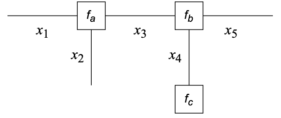
$$ f(x_1,x_2,x_3,x_4,x_5) = f_a(x_1,x_2,x_3) \cdot f_b(x_3,x_4,x_5) \cdot f_c(x_4) $$

The factorization of this function can be graphically represented by a Forney-style Factor Graph (FFG):

An FFG is an undirected graph subject to the following construction rules (Forney, 2001)
1. A node for every factor;
2. An edge (or half-edge) for every variable;
3. Node $f_\bullet$ is connected to edge $x$ iff variable $x$ appears in factor $f_\bullet$.

A configuration is an assigment of values to all variables.
A configuration $\omega=(x_1,x_2,x_3,x_4,x_5)$ is said to be valid iff $f(\omega) \neq 0$

Equality Nodes for Branching Points¶

Note that a variable can appear in maximally two factors in an FFG (since an edge has only two end points).

Consider the factorization (where $x_2$ appears in three factors)

$$ f(x_1,x_2,x_3,x_4) = f_a(x_1,x_2)\cdot f_b(x_2,x_3) \cdot f_c(x_2,x_4) $$

For the factor graph representation, we will instead consider the function $g$, defined as

$$\begin{align*} g(x_1,x_2&,x_2^\prime,x_2^{\prime\prime},x_3,x_4) = f_a(x_1,x_2)\cdot f_b(x_2^\prime,x_3) \cdot f_c(x_2^{\prime\prime},x_4) \cdot f_=(x_2,x_2^\prime,x_2^{\prime\prime}) \end{align*}$$

where $$ f_=(x_2,x_2^\prime,x_2^{\prime\prime}) \triangleq \delta(x_2-x_2^\prime)\, \delta(x_2-x_2^{\prime\prime}) $$

Note that through introduction of auxiliary variables $X_2^{\prime}$ and $X_2^{\prime\prime}$ and a factor $f_=(x_2,x_2^\prime,x_2^{\prime\prime})$, each variable in $g$ appears in maximally two factors.

The constraint $f_=(x,x^\prime,x^{\prime\prime})$ enforces that $X=X^\prime=X^{\prime\prime}$ for every valid configuration.

Since $f$ is a marginal of $g$, i.e.,

$$ f(x_1,x_2,x_3,x_4) = \iint g(x_1,x_2,x_2^\prime,x_2^{\prime\prime},x_3,x_4)\, \mathrm{d}x_2^\prime \mathrm{d}x_2^{\prime\prime} $$

it follows that any inference problem on $f$ can be executed by a corresponding inference problem on $g$, e.g., $$\begin{align*} f(x_1 \mid x_2) &\triangleq \frac{\iint f(x_1,x_2,x_3,x_4) \,\mathrm{d}x_3 \mathrm{d}x_4 }{ \int\cdots\int f(x_1,x_2,x_3,x_4) \,\mathrm{d}x_1 \mathrm{d}x_3 \mathrm{d}x_4} \\ &= \frac{\int\cdots\int g(x_1,x_2,x_2^\prime,x_2^{\prime\prime},x_3,x_4) \,\mathrm{d}x_2^\prime \mathrm{d}x_2^{\prime\prime} \mathrm{d}x_3 \mathrm{d}x_4 }{ \int\cdots\int g(x_1,x_2,x_2^\prime,x_2^{\prime\prime},x_3,x_4) \,\mathrm{d}x_1 \mathrm{d}x_2^\prime \mathrm{d}x_2^{\prime\prime} \mathrm{d}x_3 \mathrm{d}x_4} \\ &= g(x_1 \mid x_2) \end{align*}$$

$\Rightarrow$ Any factorization of a global function $f$ can be represented by a Forney-style Factor Graph.

Probabilistic Models as Factor Graphs¶

FFGs can be used to express conditional independence (factorization) in probabilistic models.

For example, the (previously shown) graph for

$f_a(x_1,x_2,x_3) \cdot f_b(x_3,x_4,x_5) \cdot f_c(x_4)$ could represent the probabilistic model $$ p(x_1,x_2,x_3,x_4,x_5) = p(x_1,x_2|x_3) \cdot p(x_3,x_5|x_4) \cdot p(x_4) $$ where we identify $$\begin{align*} f_a(x_1,x_2,x_3) &= p(x_1,x_2|x_3) \\ f_b(x_3,x_4,x_5) &= p(x_3,x_5|x_4) \\ f_c(x_4) &= p(x_4) \end{align*}$$

This is the graph

Inference by Closing Boxes¶

Factorizations provide opportunities to cut on the amount of needed computations when doing inference. In what follows, we will use FFGs to process these opportunities in an automatic way by message passing between the nodes of the graph.

Assume we wish to compute the marginal

$$ \bar{f}(x_3) \triangleq \sum\limits_{x_1,x_2,x_4,x_5,x_6,x_7}f(x_1,x_2,\ldots,x_7) $$

for a model $f$ with given factorization $$ f(x_1,x_2,\ldots,x_7) = f_a(x_1) f_b(x_2) f_c(x_1,x_2,x_3) f_d(x_4) f_e(x_3,x_4,x_5) f_f(x_5,x_6,x_7) f_g(x_7) $$

Note that, if each variable $x_i$ can take on $10$ values, then the computing the marginal $\bar{f}(x_3)$ takes about $10^6$ (1 million) additions.

Due to the factorization and the Generalized Distributive Law, we can decompose this sum-of-products to the following product-of-sums:

$$\begin{align*}\bar{f}&(x_3) = \\ &\underbrace{ \Bigg( \sum_{x_1,x_2} \underbrace{f_a(x_1)}_{\overrightarrow{\mu}_{X_1}(x_1)}\, \underbrace{f_b(x_2)}_{\overrightarrow{\mu}_{X_2}(x_2)}\,f_c(x_1,x_2,x_3)\Bigg) }_{\overrightarrow{\mu}_{X_3}(x_3)} \underbrace{ \cdot\Bigg( \sum_{x_4,x_5} \underbrace{f_d(x_4)}_{\overrightarrow{\mu}_{X_4}(x_4)}\,f_e(x_3,x_4,x_5) \cdot \underbrace{ \big( \sum_{x_6,x_7} f_f(x_5,x_6,x_7)\,\underbrace{f_g(x_7)}_{\overleftarrow{\mu}_{X_7}(x_7)}\big) }_{\overleftarrow{\mu}_{X_5}(x_5)} \Bigg) }_{\overleftarrow{\mu}_{X_3}(x_3)} \end{align*}$$

which, in case $x_i$ has $10$ values, requires a few hundred additions and is therefore computationally (much!) lighter than executing the full sum $\sum_{x_1,\ldots,x_7}f(x_1,x_2,\ldots,x_7)$

Note that the auxiliary factor $\overrightarrow{\mu}_{X_3}(x_3)$ is obtained by multiplying all enclosed factors ($f_a$, $f_b, f_c$) by the red dashed box, followed by marginalization (summing) over all enclosed variables ($x_1$, $x_2$).

This is the Closing the Box-rule, which is a general recipe for marginalization of latent variables (inside the box) and leads to a new factor that has the variables (edges) that cross the box as arguments. For instance, the argument of the remaining factor $\overrightarrow{\mu}_{X_3}(x_3)$ is the variable on the edge that crosses the red box ($x_3$).

Hence, $\overrightarrow{\mu}_{X_3}(x_3)$ can be interpreted as a message from the red box toward variable $x_3$.

We drew directed edges in the FFG in order to distinguish forward messages $\overrightarrow{\mu}_\bullet(\cdot)$ (in the same direction as the arrow of the edge) from backward messages $\overleftarrow{\mu}_\bullet(\cdot)$ (in opposite direction). This is just a notational convenience since an FFG is computationally an undirected graph.

Sum-Product Algorithm¶

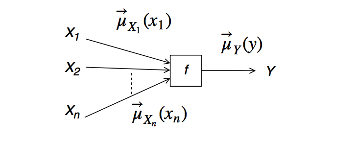
Closing-the-box can also be interpreted as a message update rule for an outgoing message from a node. For a node $f(y,x_1,\ldots,x_n)$ with incoming messages $\overrightarrow{\mu}_{X_1}(x_1), \overrightarrow{\mu}_{X_1}(x_1), \ldots,\overrightarrow{\mu}_{X_n}(x_n)$, the outgoing message is given by (Loeliger (2007), pg.1299):

$$ \boxed{ \underbrace{\overrightarrow{\mu}_{Y}(y)}_{\substack{ \text{outgoing}\\ \text{message}}} = \sum_{x_1,\ldots,x_n} \underbrace{\overrightarrow{\mu}_{X_1}(x_1)\cdots \overrightarrow{\mu}_{X_n}(x_n)}_{\substack{\text{incoming} \\ \text{messages}}} \cdot \underbrace{f(y,x_1,\ldots,x_n)}_{\substack{\text{node}\\ \text{function}}} } $$

This is called the Sum-Product Message (SPM) update rule. (Look at the formula to understand why it's called the SPM update rule).

Note that all SPM update rules can be computed from information that is locally available at each node.

If the factor graph for a function $f$ has no cycles (i.e., the graph is a tree), then the marginal $\bar{f}(x_3) = \sum_{x_1,x_2,x_4,x_5,x_6,x_7}f(x_1,x_2,\ldots,x_7)$ is given by multiplying the forward and backward messages on that edge:

$$ \boxed{ \bar{f}(x_3) = \overrightarrow{\mu}_{X_3}(x_3)\cdot \overleftarrow{\mu}_{X_3}(x_3)} $$

It follows that the marginal $\bar{f}(x_3) = \sum_{x_1,x_2,x_4,x_5,x_6,x_7}f(x_1,x_2,\ldots,x_7)$ can be efficiently computed through sum-product messages. Executing inference through SP message passing is called the Sum-Product Algorithm (or alternatively, the belief propagation algorithm).

Just as a final note, inference by sum-product message passing is much like replacing the sum-of-products

$$ ac + ad + bc + bd$$

by the following product-of-sums: $$ (a + b)(c + d) \,.$$

Which of these two computations is cheaper to execute?

Sum-Product Messages for the Equality Node ¶

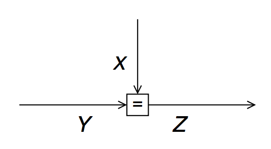
As an example, let´s evaluate the SP messages for the equality node $f_=(x,y,z) = \delta(z-x)\delta(z-y)$:

$$\begin{align*} \overrightarrow{\mu}_{Z}(z) &= \iint \overrightarrow{\mu}_{X}(x) \overrightarrow{\mu}_{Y}(y) \,\delta(z-x)\delta(z-y) \,\mathrm{d}x \mathrm{d}y \\ &= \overrightarrow{\mu}_{X}(z) \int \overrightarrow{\mu}_{Y}(y) \,\delta(z-y) \,\mathrm{d}y \\ &= \overrightarrow{\mu}_{X}(z) \overrightarrow{\mu}_{Y}(z) \end{align*}$$

By symmetry, this also implies (for the same equality node) that

$$\begin{align*} \overleftarrow{\mu}_{X}(x) &= \overrightarrow{\mu}_{Y}(x) \overleftarrow{\mu}_{Z}(x) \quad \text{and} \\ \overleftarrow{\mu}_{Y}(y) &= \overrightarrow{\mu}_{X}(y) \overleftarrow{\mu}_{Z}(y)\,. \end{align*}$$

Let us now consider the case of Gaussian messages $\overrightarrow{\mu}_{X}(x) = \mathcal{N}(x|\overrightarrow{m}_X,\overrightarrow{V}_X)$, $\overrightarrow{\mu}_{Y}(y) = \mathcal{N}(y| \overrightarrow{m}_Y,\overrightarrow{V}_Y)$ and $\overrightarrow{\mu}_{Z}(z) = \mathcal{N}(z|\overrightarrow{m}_Z,\overrightarrow{V}_Z)$. Let´s also define the precision matrices $\overrightarrow{W}_X \triangleq \overrightarrow{V}_X^{-1}$ and similarly for $Y$ and $Z$. Then applying the SP update rule leads to multiplication of two Gaussian distributions (see Roweis notes), resulting in

$$\begin{align*} \overrightarrow{W}_Z &= \overrightarrow{W}_X + \overrightarrow{W}_Y \qquad &\text{(precisions add)}\\ \overrightarrow{W}_Z \overrightarrow{m}_z &= \overrightarrow{W}_X \overrightarrow{m}_X + \overrightarrow{W}_Y \overrightarrow{m}_Y \qquad &\text{(natural means add)} \end{align*}$$

It follows that message passing through an equality node is similar to applying Bayes rule, i.e., fusion of two information sources. Does this make sense?

Message Passing Schedules¶

In a non-cyclic (ie, tree) graph, start with messages from the terminals and keep passing messages through the internal nodes towards the "target" variable ($x_3$ in above problem) until you have both the forward and backward message for the target variable.

In a tree graph, if you continue to pass messages throughout the graph, the Sum-Product Algorithm computes exact marginals for all hidden variables.

If the graph contains cycles, we have in principle an infinite tree by "unrolling" the graph. In this case, the SP Algorithm is not guaranteed to find exact marginals. In practice, if we apply the SP algorithm for just a few iterations ("unrolls"), then we often find satisfying approximate marginals.

Terminal Nodes and Processing Observations¶

We can use terminal nodes to represent observations, e.g., add a factor $f(y)=\delta(y−3)$ to terminate the half-edge for variable $Y$ if $y=3$ is observed.

Terminal nodes that carry observations are denoted by small black boxes.

The message out of a terminal node (attached to only 1 edge) is the factor itself. For instance, closing a box around terminal node $f_a(x_1)$ would lead to $$\overrightarrow{\mu}_{X_1}(x_1) \triangleq \sum_{ \stackrel{ \textrm{enclosed} }{ \textrm{variables} } } \;\prod_{\stackrel{ \textrm{enclosed} }{ \textrm{factors} }} f_a(x_1) = f_a(x_1)\,$$

since there are no enclosed variables.

The message from a half-edge is $1$ (one). You can verify this by imagining that a half-edge $x$ can be terminated by a node function $f(x)=1$ without affecting any inference issue.

Automating Bayesian Inference by Message Passing¶

The foregoing message update rules can be worked out in closed-form and put into tables (e.g., see Tables 1 through 6 in Loeliger (2007) for many standard factors such as essential probability distributions and operations such as additions, fixed-gain multiplications and branching (equality nodes).
In the optional slides below, we have worked out a few more update rules for the addition node and the multiplication node.
If the update rules for all node types in a graph have been tabulated, then inference by message passing comes down to executing a set of table-lookup operations, thus creating a completely automatable Bayesian inference framework.
In our research lab BIASlab (FLUX 7.060), we are developing RxInfer, which is a (Julia) toolbox for automating Bayesian inference by message passing in a factor graph.

Example: Bayesian Linear Regression by Message Passing¶

Assume we want to estimate some function $f: \mathbb{R}^D \rightarrow \mathbb{R}$ from a given data set $D = \{(x_1,y_1), \ldots, (x_N,y_N)\}$, with model assumption $y_i = f(x_i) + \epsilon_i$.

model specification¶

We will assume a linear model with white Gaussian noise and a Gaussian prior on the coefficients $w$:

$$\begin{align*} y_i &= w^T x_i + \epsilon_i \\ \epsilon_i &\sim \mathcal{N}(0, \sigma^2) \\ w &\sim \mathcal{N}(0,\Sigma) \end{align*}$$

or equivalently $$\begin{align*} p(w,\epsilon,D) &= \overbrace{p(w)}^{\text{weight prior}} \prod_{i=1}^N \overbrace{p(y_i\,|\,x_i,w,\epsilon_i)}^{\text{regression model}} \overbrace{p(\epsilon_i)}^{\text{noise model}} \\ &= \mathcal{N}(w\,|\,0,\Sigma) \prod_{i=1}^N \delta(y_i - w^T x_i - \epsilon_i) \mathcal{N}(\epsilon_i\,|\,0,\sigma^2) \end{align*}$$

Inference (parameter estimation)¶

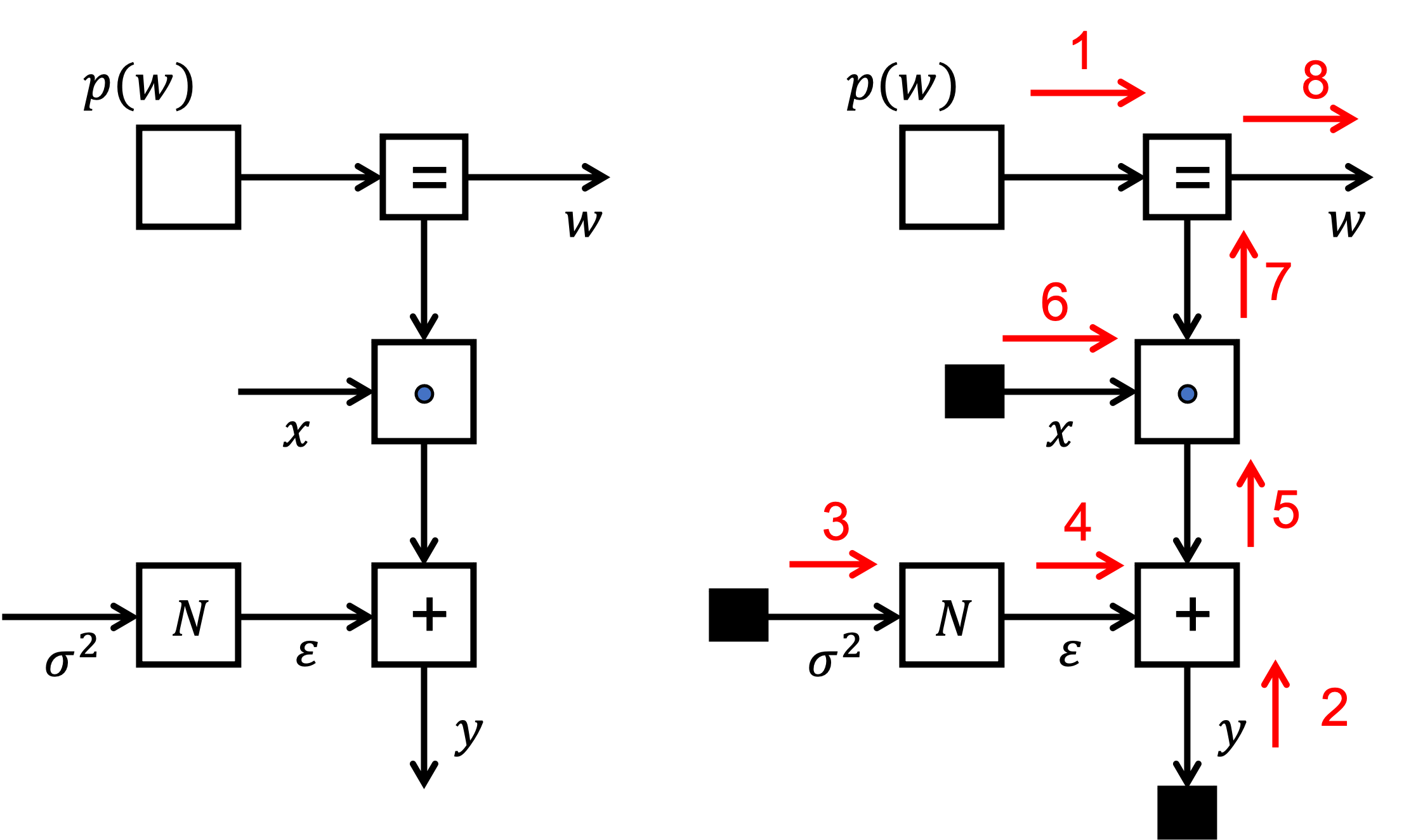
We are interested in inferring the posterior $p(w|D)$. We will execute inference by message passing on the FFG for the model.

The left figure shows the factor graph for this model.
The right figure shows the message passing scheme.

CODE EXAMPLE¶

Let's solve this problem by message passing-based inference with Julia's FFG toolbox RxInfer.

In [ ]:

using Pkg; Pkg.activate("../."); Pkg.instantiate();
using IJulia; try IJulia.clear_output(); catch _ end

In [2]:

using Plots, LinearAlgebra, LaTeXStrings

# Parameters
Σ = 1e5 * Diagonal(I,3) # Covariance matrix of prior on w
σ2 = 2.0                # Noise variance

# Generate data set
w = [1.0; 2.0; 0.25]
N = 30
z = 10.0*rand(N)
x_train = [[1.0; z; z^2] for z in z] # Feature vector x = [1.0; z; z^2]
f(x) = (w'*x)[1]
y_train = map(f, x_train) + sqrt(σ2)*randn(N) # y[i] = w' * x[i] + ϵ
scatter(z, y_train, label="data", xlabel=L"z", ylabel=L"f([1.0, z, z^2]) + \epsilon")

Now build the factor graph in RxInfer, perform sum-product message passing and plot results (mean of posterior).

In [3]:

using RxInfer, Random
# Build model
@model function linear_regression(y,x, N, Σ, σ2)

    w ~ MvNormalMeanCovariance(zeros(3),Σ)
    
    for i in 1:N
        y[i] ~ NormalMeanVariance(dot(w , x[i]), σ2)
    end
end
# Run message passing algorithm 
results = infer(
    model      = linear_regression(N=length(x_train), Σ=Σ, σ2=σ2),
    data       = (y = y_train, x = x_train),
    returnvars = (w = KeepLast(),),
    iterations = 20,
);
# Plot result
w = results.posteriors[:w]
println("Posterior distribution of w: $(w)")
plt = scatter(z, y_train, label="data", xlabel=L"z", ylabel=L"f([1.0, z, z^2]) + \epsilon")
z_test = collect(0:0.2:12)
x_test = [[1.0; z; z^2] for z in z_test]
for i=1:10
    w_sample = rand(results.posteriors[:w])
    f_est(x) = (w_sample'*x)[1]
    plt = plot!(z_test, map(f_est, x_test), alpha=0.3, label="");
end
display(plt)

Posterior distribution of w: MvNormalWeightedMeanPrecision(
xi: [307.7818564544745, 2208.395106150794, 17693.181354856355]
Λ: [15.00001 77.73321536791191 538.9138576517117; 77.73321536791191 538.9138676517117 4221.088404002255; 538.9138576517117 4221.088404002255 35248.048308516314]
)

Final thoughts: Modularity and Abstraction¶

The great Michael Jordan (no, not this one, but this one), wrote:

"I basically know of two principles for treating complicated systems in simple ways: the first is the principle of modularity and the second is the principle of abstraction. I am an apologist for computational probability in machine learning because I believe that probability theory implements these two principles in deep and intriguing ways — namely through factorization and through averaging. Exploiting these two mechanisms as fully as possible seems to me to be the way forward in machine learning." — Michael Jordan, 1997 (quoted in Fre98).
Factor graphs realize these ideas nicely, both visually and computationally.
Visually, the modularity of conditional independencies in the model are displayed by the graph structure. Each node hides internal complexity and by closing-the-box, we can hierarchically move on to higher levels of abstraction.
Computationally, message passing-based inference uses the Distributive Law to avoid any unnecessary computations.
What is the relevance of this lesson? RxInfer is not yet a finished project. Still, my prediction is that in 5-10 years, this lesson on Factor Graphs will be the final lecture of part-A of this class, aimed at engineers who need to develop machine learning applications. In principle you have all the tools now to work out the 4-step machine learning recipe (1. model specification, 2. parameter learning, 3. model evaluation, 4. application) that was proposed in the Bayesian machine learning lesson. You can propose any model and execute the (learning, evaluation, and application) stages by executing the corresponding inference task automatically in RxInfer.
Part-B of this class would be about on advanced methods on how to improve automated inference by RxInfer or a similar probabilistic programming package. The Bayesian approach fully supports separating model specification from the inference task.

OPTIONAL SLIDES¶

Sum-Product Messages for Multiplication Nodes ¶

Next, let us consider a multiplication by a fixed (invertible matrix) gain $f_A(x,y) = \delta(y-Ax)$

$$\begin{align*} \overrightarrow{\mu}_{Y}(y) &= \int \overrightarrow{\mu}_{X}(x) \,\delta(y-Ax) \,\mathrm{d}x \\ &= \int \overrightarrow{\mu}_{X}(x) \,|A|^{-1}\delta(x-A^{-1}y) \,\mathrm{d}x \\ &= |A|^{-1}\overrightarrow{\mu}_{X}(A^{-1}y) \,. \end{align*}$$

For a Gaussian message input message $\overrightarrow{\mu}_{X}(x) = \mathcal{N}(x|\overrightarrow{m}_{X},\overrightarrow{V}_{X})$, the output message is also Gaussian with

$$\begin{align*} \overrightarrow{m}_{Y} = A\overrightarrow{m}_{X} \,,\,\text{and}\,\, \overrightarrow{V}_{Y} = A\overrightarrow{V}_{X}A^T \end{align*}$$

since $$\begin{align*} \overrightarrow{\mu}_{Y}(y) &= |A|^{-1}\overrightarrow{\mu}_{X}(A^{-1}y) \\ &\propto \exp \left( -\frac{1}{2} \left( A^{-1}y - \overrightarrow{m}_{X}\right)^T \overrightarrow{V}_{X}^{-1} \left( A^{-1}y - \overrightarrow{m}_{X}\right)\right) \\ &= \exp \big( -\frac{1}{2} \left( y - A\overrightarrow{m}_{X}\right)^T \underbrace{A^{-T}\overrightarrow{V}_{X}^{-1} A^{-1}}_{(A \overrightarrow{V}_{X} A^T)^{-1}} \left( y - A\overrightarrow{m}_{X}\right)\big) \\ &\propto \mathcal{N}(y| A\overrightarrow{m}_{X},A\overrightarrow{V}_{X}A^T) \,. \end{align*}$$

Exercise: Proof that, for the same factor $\delta(y-Ax)$ and Gaussian messages, the (backward) sum-product message $\overleftarrow{\mu}_{X}$ is given by

$$\begin{align*} \overleftarrow{\xi}_{X} &= A^T\overleftarrow{\xi}_{Y} \\ \overleftarrow{W}_{X} &= A^T\overleftarrow{W}_{Y}A \end{align*}$$

where $\overleftarrow{\xi}_X \triangleq \overleftarrow{W}_X \overleftarrow{m}_X$ and $\overleftarrow{W}_{X} \triangleq \overleftarrow{V}_{X}^{-1}$ (and similarly for $Y$).

Code example: Gaussian forward and backward messages for the Addition node¶

Let's calculate the Gaussian forward and backward messages for the addition node in RxInfer.

In [4]:

println("Forward message on Z:")
@call_rule typeof(+)(:out, Marginalisation) (m_in1 = NormalMeanVariance(1.0, 1.0), m_in2 = NormalMeanVariance(2.0, 1.0))

Forward message on Z:

WARNING: both ExponentialFamily and ReactiveMP export "MvNormalMeanScalePrecision"; uses of it in module RxInfer must be qualified

NormalMeanVariance{Float64}(μ=3.0, v=2.0)

In [5]:

println("Backward message on X:")
@call_rule typeof(+)(:in1, Marginalisation) (m_out = NormalMeanVariance(3.0, 1.0), m_in2 = NormalMeanVariance(2.0, 1.0))

Backward message on X:

NormalMeanVariance{Float64}(μ=1.0, v=2.0)

Code Example: forward and backward messages for the Matrix Multiplication node¶

In the same way we can also investigate the forward and backward messages for the matrix multiplication ("gain") node

In [6]:

println("Forward message on Y:")
@call_rule typeof(*)(:out, Marginalisation) (m_A = PointMass(4.0), m_in = NormalMeanVariance(1.0, 1.0))

Forward message on Y:

NormalMeanVariance{Float64}(μ=4.0, v=16.0)

In [7]:

println("Backward message on X:")
@call_rule typeof(*)(:in, Marginalisation) (m_out = NormalMeanVariance(2.0, 1.0), m_A = PointMass(4.0))

Backward message on X:

NormalWeightedMeanPrecision{Float64}(xi=8.0, w=16.0)

Example: Sum-Product Algorithm to infer a posterior¶

Consider a generative model

$$p(x,y_1,y_2) = p(x)\,p(y_1|x)\,p(y_2|x) .$$

This model expresses the assumption that $Y_1$ and $Y_2$ are independent measurements of $X$.

Assume that we are interested in the posterior for $X$ after observing $Y_1= \hat y_1$ and $Y_2= \hat y_2$. The posterior for $X$ can be inferred by applying the sum-product algorithm to the following graph:

(Note that) we usually draw terminal nodes for observed variables in the graph by smaller solid-black squares. This is just to help the visualization of the graph, since the computational rules are no different than for other nodes.

Code for Sum-Product Algorithm to infer a posterior¶

We'll use RxInfer to build the above graph, and perform sum-product message passing to infer the posterior $p(x|y_1,y_2)$. We assume $p(y_1|x)$ and $p(y_2|x)$ to be Gaussian likelihoods with known variances: $$\begin{align*} p(y_1\,|\,x) &= \mathcal{N}(y_1\,|\,x, v_{y1}) \\ p(y_2\,|\,x) &= \mathcal{N}(y_2\,|\,x, v_{y2}) \end{align*}$$ Under this model, the posterior is given by: $$\begin{align*} p(x\,|\,y_1,y_2) &\propto \overbrace{p(y_1\,|\,x)\,p(y_2\,|\,x)}^{\text{likelihood}}\,\overbrace{p(x)}^{\text{prior}} \\ &=\mathcal{N}(x\,|\,\hat{y}_1, v_{y1})\, \mathcal{N}(x\,|\,\hat{y}_2, v_{y2}) \, \mathcal{N}(x\,|\,m_x, v_x) \end{align*}$$ so we can validate the answer by solving the Gaussian multiplication manually.

In [ ]:

# Data
y1_hat = 1.0
y2_hat = 2.0

# Construct the factor graph
@model function my_model(y1,y2)

    # `x` is the hidden states
    x ~ NormalMeanVariance(0.0, 4.0)

    # `y1` and `y2` are "clamped" observations
    y1 ~ NormalMeanVariance(x, 1.0)
    y2 ~ NormalMeanVariance(x, 2.0)
    
    return x
end

result = infer(model=my_model(), data=(y1=y1_hat, y2 = y2_hat,))
println("Sum-product message passing result: p(x|y1,y2) = 𝒩($(mean(result.posteriors[:x])),$(var(result.posteriors[:x])))")

# Calculate mean and variance of p(x|y1,y2) manually by multiplying 3 Gaussians (see lesson 4 for details)
v = 1 / (1/4 + 1/1 + 1/2)
m = v * (0/4 + y1_hat/1.0 + y2_hat/2.0)
println("Manual result: p(x|y1,y2) = 𝒩($(m), $(v))")

In [ ]:

open("../../styles/aipstyle.html") do f display("text/html", read(f, String)) end

Factor Graphs¶

Preliminaries¶

Why Factor Graphs?¶

Factor Graph Construction Rules¶

Equality Nodes for Branching Points¶

Probabilistic Models as Factor Graphs¶

Inference by Closing Boxes¶

Sum-Product Algorithm¶

Sum-Product Messages for the Equality Node¶

Message Passing Schedules¶

Terminal Nodes and Processing Observations¶

Automating Bayesian Inference by Message Passing¶

Example: Bayesian Linear Regression by Message Passing¶

model specification¶

Inference (parameter estimation)¶

CODE EXAMPLE¶

Final thoughts: Modularity and Abstraction¶

OPTIONAL SLIDES¶

Sum-Product Messages for Multiplication Nodes¶

Code example: Gaussian forward and backward messages for the Addition node¶

Code Example: forward and backward messages for the Matrix Multiplication node¶

Example: Sum-Product Algorithm to infer a posterior¶

Code for Sum-Product Algorithm to infer a posterior¶

Sum-Product Messages for the Equality Node ¶

Sum-Product Messages for Multiplication Nodes ¶