Dynamic Models
Preliminaries
- Goal
- Introduction to dynamic (=temporal) Latent Variable Models, including the Hidden Markov Model and Kalman filter.
- Materials
- Mandatory
- These lecture notes
- Optional
- Bishop pp.605-615 on Hidden Markov Models
- Bishop pp.635-641 on Kalman filters
- Faragher (2012), Understanding the Basis of the Kalman Filter
- Minka (1999), From Hidden Markov Models to Linear Dynamical Systems
- Mandatory
Example Problem
We consider a one-dimensional cart position tracking problem, see Faragher 2012.
The hidden states are the position $z_t$ and velocity $\dot z_t$. We can apply an external acceleration/breaking force $u_t$. (Noisy) observations are represented by $x_t$.
The equations of motions are given by
- Task: Infer the position $z_t$ after 10 time steps. (Solution later in this lesson).

Dynamical Models
In this lesson, we consider models where the sequence order of observations matters.
Consider the ordered observation sequence $x^T \triangleq \left(x_1,x_2,\ldots,x_T\right)$.
- (For brevity, in this lesson we use the notation $x_t^T$ to denote $(x_t,x_{t+1},\ldots,x_T)$ and drop the subscript if $t=1$, so $x^T = x_1^T = \left(x_1,x_2,\ldots,x_T\right)$).
- We wish to develop a generative model $$ p( x^T )$$
that 'explains' the time series $x^T$.
- We cannot use the IID assumption $p( x^T ) = \prod_t p(x_t )$. In general, we can use the chain rule (a.k.a. the general product rule)
- Generally, we will want to limit the depth of dependencies on previous observations. For example, a $K$th-order linear Auto-Regressive (AR) model that is given by
limits the dependencies to the past $K$ samples.
State-space Models
- A limitation of AR models is that they need a lot of parameters in order to create a flexible model. E.g., if $x_t$ is an $M$-dimensional discrete variable, then a $K$th-order AR model will have about $M^{K}$ parameters.
- Similar to our work on Gaussian Mixture models, we can create a flexible dynamic system by introducing latent (unobserved) variables $z^T \triangleq \left(z_1,z_2,\dots,z_T\right)$ (one $z_t$ for each observation $x_t$). In dynamic systems, $z_t$ are called state variables.
- A state space model is a particular latent variable dynamical model defined by
- The condition $p(z_t\,|\,z^{t-1}) = p(z_t\,|\,z_{t-1})$ is called a $1$st-order Markov condition.
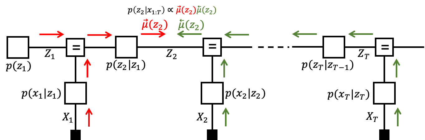
- The Forney-style factor graph for a state-space model:

Hidden Markov Models and Linear Dynamical Systems
- A Hidden Markov Model (HMM) is a specific state-space model with discrete-valued state variables $z_t$.
- Typically, $z_t$ is a $K$-dimensional one-hot coded latent 'class indicator' with transition probabilities $a_{jk} \triangleq p(z_{tk}=1\,|\,z_{t-1,j}=1)$, or equivalently, $$p(z_t|z_{t-1}) = \prod_{k=1}^K \prod_{j=1}^K a_{jk}^{z_{t-1,j}\cdot z_{tk}}$$
which is usually accompanied by an initial state distribution $p(z_{1k}=1) = \pi_k$.
- The classical HMM has also discrete-valued observations but in pratice any (probabilistic) observation model $p(x_t|z_t)$ may be coupled to the hidden Markov chain.
- Another well-known state-space model with continuous-valued state variables $z_t$ is the (Linear) Gaussian Dynamical System (LGDS), which is defined as
- Note that the joint distribution over all states and observations $\{(x_1,z_1),\ldots,(x_t,z_t)\}$ is a (large-dimensional) Gaussian distribution. This means that, in principle, every inference problem on the LGDS model also leads to a Gaussian distribution.
- HMM's and LGDS's (and variants thereof) are at the basis of a wide range of complex information processing systems, such as speech and language recognition, robotics and automatic car navigation, and even processing of DNA sequences.
Common Signal Processing Tasks as Message Passing-based Inference
As we have seen, inference tasks in linear Gaussian state space models can be analytically solved.
However, these derivations quickly become cumbersome and prone to errors.
Alternatively, we could specify the generative model in a (Forney-style) factor graph and use automated message passing to infer the posterior over the hidden variables. Here follows some examples.
Filtering, a.k.a. state estimation: estimation of a state (at time step $t$), based on past and current (at $t$) observations.

- Smoothing: estimation of a state based on both past and future observations. Needs backward messages from the future.
- Prediction: estimation of future state or observation based only on observations of the past.

Kalman Filtering
- Technically, a Kalman filter is the solution to the recursive estimation (inference) of the hidden state $z_t$ based on past observations in an LGDS, i.e., Kalman filtering solves the problem $p(z_t\,|\,x^t)$ based on the previous estimate $p(z_{t-1}\,|\,x^{t-1})$ and a new observation $x_t$ (in the context of the given model specification of course).
- Let's infer the Kalman filter for a scalar linear Gaussian dynamical system:
- Kalman filtering comprises inferring $p(z_t\,|\,x^t)$ from a given prior estimate $p(z_{t-1}\,|\,x^{t-1})$ (available after the previous time step) and a new observation $x_t$. Let us assume that
- Note that everything is Gaussian, so it is in principle possible to execute inference problems analytically and the result will be a Gaussian posterior:
- (In the following derivation we make use of the renormalization equality $\mathcal{N}(x\,|\,cz,\sigma^2) = \frac{1}{c}\mathcal{N}\left(z \,\big|\,\frac{x}{c},\left(\frac{\sigma}{c}\right)^2\right)$).
with $$\begin{align*} \rho_t^2 &= a^2 \sigma_{t-1}^2 + \sigma_z^2 \tag{predicted variance}\\ K_t &= \frac{c \rho_t^2}{c^2 \rho_t^2 + \sigma_x^2} \tag{Kalman gain} \\ \mu_t &= \underbrace{a \mu_{t-1}}_{\text{prior prediction}} + K_t \cdot \underbrace{\left( x_t - c a \mu_{t-1}\right)}_{\text{prediction error}} \tag{posterior mean}\\ \sigma_t^2 &= \left( 1 - c\cdot K_t \right) \rho_t^2 \tag{posterior variance} \end{align*}$$
Kalman filtering consists of computing/updating these last four equations for each new observation ($x_t$). This is a very efficient recursive algorithm to estimate the state $z_t$ from all observations (until $t$).
It turns out that it's also possible to get an analytical result for $p(x_t|x^{t-1})$, which is the model evidence in a filtering context. See optional slides for details.
Multi-dimensional Kalman Filtering
- The Kalman filter equations can also be derived for multidimensional state-space models. In particular, for the model
the Kalman filter update equations for the posterior $p(z_t |x^t) = \mathcal{N}\left(z_t \bigm| \mu_t, V_t \right)$ are given by (see Bishop, pg.639) $$\begin{align*} P_t &= A V_{t-1} A^T + \Gamma \tag{predicted variance}\\ K_t &= P_t C^T \cdot \left(C P_t C^T + \Sigma \right)^{-1} \tag{Kalman gain} \\ \mu_t &= A \mu_{t-1} + K_t\cdot\left(x_t - C A \mu_{t-1} \right) \tag{posterior state mean}\\ V_t &= \left(I-K_t C \right) P_{t} \tag{posterior state variance} \end{align*}$$
Code Example: Kalman Filtering and the Cart Position Tracking Example Revisited
- We can now solve the cart tracking problem of the introductory example by implementing the Kalman filter.
using Pkg;Pkg.activate("probprog/workspace/");Pkg.instantiate()
IJulia.clear_output();
using LinearAlgebra, PyPlot
include("scripts/cart_tracking_helpers.jl")

# Specify the model parameters
Δt = 1.0                     # assume the time steps to be equal in size
A = [1.0 Δt;
     0.0 1.0]
b = [0.5*Δt^2; Δt]
Σz = convert(Matrix,Diagonal([0.2*Δt; 0.1*Δt])) # process noise covariance
Σx = convert(Matrix,Diagonal([1.0; 2.0]))     # observation noise covariance;

# Generate noisy observations
n = 10                # perform 10 timesteps
z_start = [10.0; 2.0] # initial state
u = 0.2 * ones(n)     # constant input u
noisy_x = generateNoisyMeasurements(z_start, u, A, b, Σz, Σx);

m_z = noisy_x[1]                                    # initial predictive mean
V_z = A * (1e8*Diagonal(I,2) * A') + Σz             # initial predictive covariance

for t = 2:n
    global m_z, V_z, m_pred_z, V_pred_z
    #predict
    m_pred_z = A * m_z + b * u[t]                   # predictive mean
    V_pred_z = A * V_z * A' + Σz                    # predictive covariance
    #update
    gain = V_pred_z * inv(V_pred_z + Σx)            # Kalman gain
    m_z = m_pred_z + gain * (noisy_x[t] - m_pred_z) # posterior mean update
    V_z = (Diagonal(I,2)-gain)*V_pred_z             # posterior covariance update
end
println("Prediction: ",ProbabilityDistribution(Multivariate,GaussianMeanVariance,m=m_pred_z,v=V_pred_z))
println("Measurement: ", ProbabilityDistribution(Multivariate,GaussianMeanVariance,m=noisy_x[n],v=Σx))
println("Posterior: ", ProbabilityDistribution(Multivariate,GaussianMeanVariance,m=m_z,v=V_z))
plotCartPrediction2(m_pred_z[1], V_pred_z[1], m_z[1], V_z[1], noisy_x[n][1], Σx[1][1]);
Prediction: 𝒩(m=[42.21, 4.51], v=[[1.30, 0.39][0.39, 0.34]])

Measurement: 𝒩(m=[40.88, 5.41], v=[[1.00, 0.00][0.00, 2.00]])

Posterior: 𝒩(m=[41.55, 4.42], v=[[0.55, 0.15][0.15, 0.24]])
The Cart Tracking Problem Revisited: Inference by Message Passing
- Let's solve the cart tracking problem by sum-product message passing in a factor graph like the one depicted above. All we have to do is create factor nodes for the state-transition model $p(z_t|z_{t-1})$ and the observation model $p(x_t|z_t)$. Then we just build the factor graph and let ForneyLab execute the message passing schedule.
- Since the factor graph is just a concatination of $n$ identical "sections" (one for each time step), we only have to specify a single section. When running the message passing algorithm we will explictly use the posterior of the previous timestep as prior in the next one. Let's build a section of the factor graph:
fg = FactorGraph()
z_prev_m = Variable(id=:z_prev_m); placeholder(z_prev_m, :z_prev_m, dims=(2,))
z_prev_v = Variable(id=:z_prev_v); placeholder(z_prev_v, :z_prev_v, dims=(2,2))
bu = Variable(id=:bu); placeholder(bu, :bu, dims=(2,))

@RV z_prev ~ GaussianMeanVariance(z_prev_m, z_prev_v, id=:z_prev) # p(z_prev)
@RV noise_z ~ GaussianMeanVariance(constant(zeros(2), id=:noise_z_m), constant(Σz, id=:noise_z_v)) # process noise
@RV z = constant(A, id=:A) * z_prev + bu + noise_z; z.id = :z # p(z|z_prev) (state transition model)
@RV x ~ GaussianMeanVariance(z, constant(Σx, id=:Σx)) # p(x|z) (observation model)
placeholder(x, :x, dims=(2,));
ForneyLab.draw(fg)
Now that we've built the factor graph, we can perform Kalman filtering by inserting measurement data into the factor graph and performing message passing.
include("scripts/cart_tracking_helpers.jl")
algo = messagePassingAlgorithm(z)
source_code = algorithmSourceCode(algo)
eval(Meta.parse(source_code))
marginals = Dict()
messages = Array{Message}(undef,6)
z_prev_m_0 = noisy_x[1]
z_prev_v_0 = A * (1e8*Diagonal(I,2) * A') + Σz
for t=2:n
    data = Dict(:x => noisy_x[t], :bu => b*u[t],:z_prev_m => z_prev_m_0, :z_prev_v => z_prev_v_0)
    step!(data, marginals, messages) # perform msg passing (single timestep)
    # Posterior of z becomes prior of z in the next timestep:
    z_prev_m_0 = ForneyLab.unsafeMean(marginals[:z])
    z_prev_v_0 = ForneyLab.unsafeCov(marginals[:z])
end
# Collect prediction p(z[n]|z[n-1]), measurement p(z[n]|x[n]), corrected prediction p(z[n]|z[n-1],x[n])
prediction      = messages[5].dist # the message index is found by manual inspection of the schedule
measurement     = messages[6].dist
corr_prediction = convert(ProbabilityDistribution{Multivariate, GaussianMeanVariance}, marginals[:z])
println("Prediction: ",prediction)
println("Measurement: ",measurement)
println("Posterior: ", corr_prediction)

# Make a fancy plot of the prediction, noisy measurement, and corrected prediction after n timesteps
plotCartPrediction(prediction, measurement, corr_prediction);

Prediction: 𝒩(m=[42.21, 4.51], v=[[1.30, 0.39][0.39, 0.34]])

Measurement: 𝒩(m=[40.88, 5.41], v=[[1.00, 0.00][0.00, 2.00]])

Posterior: 𝒩(m=[41.55, 4.42], v=[[0.55, 0.15][0.15, 0.24]])
- Note that both the analytical Kalman filtering solution and the message passing solution lead to the same results. The advantage of message passing-based inference with ForneyLab is that we did not need to derive any inference equations. ForneyLab took care of all that.
Recap Dynamical Models
- Dynamical systems do not obey the sample-by-sample independence assumption, but still can be specified, and state and parameter estimation equations can be solved by similar tools as for static models.
- Two of the more famous and powerful models with latent states include the hidden Markov model (with discrete states) and the Linear Gaussian dynamical system (with continuous states).
- For the LGDS, the Kalman filter is a well-known recursive state estimation procedure. The Kalman filter can be derived through Bayesian update rules on Gaussian distributions.
- If anything changes in the model, e.g., the state noise is not Gaussian, then you have to re-derive the inference equations again from scratch and it may not lead to an analytically pleasing answer.
- $\Rightarrow$ Generally, we will want to automate the inference processes. As we discussed, message passing in a factor graph is a visually appealing method to automate inference processes. We showed how Kalman filtering emerged naturally by automated message passing.
OPTIONAL SLIDES 
Proof of Kalman filtering equations including evidence updating
- Now let's proof the Kalman filtering equations including evidence updating by probabilistic calculus:
- The posterior $p(z_t\,|\,x^t)$ is proportional to the numerator, which by making use of the renormalization equality
can be evaluated with Gaussian multiplication rules:
$$\begin{align*} \mathcal{N}(x_t|c z_t, &\sigma_x^2) \, \sum_{z_{t-1}} \underbrace{\mathcal{N}(z_t\,|\,a z_{t-1},\sigma_z^2)}_{\text{use renormalization}} \mathcal{N}(z_{t-1} \,|\, \mu_{t-1}, \sigma_{t-1}^2) \\ &= \mathcal{N}(x_t|c z_t, \sigma_x^2) \, \sum_{z_{t-1}} \frac{1}{a}\underbrace{\mathcal{N}\left(z_{t-1}\bigm| \frac{z_t}{a},\left(\frac{\sigma_z}{a}\right)^2 \right) \mathcal{N}(z_{t-1} \,|\, \mu_{t-1}, \sigma_{t-1}^2)}_{\text{use Gaussian multiplication formula SRG-6}} \\ &= \frac{1}{a} \mathcal{N}(x_t|c z_t, \sigma_x^2) \, \sum_{z_{t-1}} \underbrace{\mathcal{N}\left(\mu_{t-1}\bigm| \frac{z_t}{a},\left(\frac{\sigma_z}{a}\right)^2 + \sigma_{t-1}^2 \right)}_{\text{not a function of }z_{t-1}} \underbrace{\mathcal{N}(z_{t-1} \,|\, \cdot, \cdot)}_{\text{sums to }1} \\ &= \frac{1}{a} \underbrace{\mathcal{N}(x_t|c z_t, \sigma_x^2)}_{\text{use renormalization rule}} \, \underbrace{\mathcal{N}\left(\mu_{t-1}\bigm| \frac{z_t}{a},\left(\frac{\sigma_z}{a}\right)^2 + \sigma_{t-1}^2 \right)}_{\text{use renormalization rule}} \\ &= \frac{1}{c} \underbrace{\mathcal{N}\left(z_t \bigm| \frac{x_t}{c}, \left( \frac{\sigma_x}{c}\right)^2 \right) \mathcal{N}\left(z_t\, \bigm|\,a \mu_{t-1},\sigma_z^2 + \left(a \sigma_{t-1}\right)^2 \right)}_{\text{use SRG-6 again}} \\ &= \underbrace{\frac{1}{c} \mathcal{N}\left( \frac{x_t}{c} \bigm| a \mu_{t-1}, \left( \frac{\sigma_x}{c}\right)^2+ \sigma_z^2 + \left(a \sigma_{t-1}\right)^2\right)}_{\text{use renormalization}} \, \mathcal{N}\left( z_t \,|\, \mu_t, \sigma_t^2\right)\\ &= \underbrace{\mathcal{N}\left(x_t \,|\, ca \mu_{t-1}, \sigma_x^2 + c^2(\sigma_z^2+a^2\sigma_{t-1}^2) \right)}_{\text{evidence } p(x_t|x^{t-1})} \underbrace{\mathcal{N}\left( z_t \,|\, \mu_t, \sigma_t^2\right)}_{\text{posterior }p(z_t|x^t) } \end{align*}$$with $$\begin{align*} \rho_t^2 &= a^2 \sigma_{t-1}^2 + \sigma_z^2 \tag{predicted variance}\\ K_t &= \frac{c \rho_t^2}{c^2 \rho_t^2 + \sigma_x^2} \tag{Kalman gain} \\ \mu_t &= \underbrace{a \mu_{t-1}}_{\text{prior prediction}} + K_t \cdot \underbrace{\left( x_t - c a \mu_{t-1}\right)}_{\text{prediction error}} \tag{posterior mean}\\ \sigma_t^2 &= \left( 1 - c\cdot K_t \right) \rho_t^2 \tag{posterior variance} \end{align*}$$
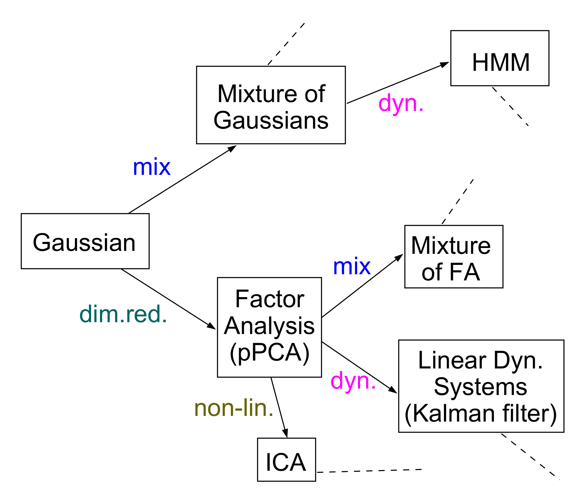
Extensions of Generative Gaussian Models
- Using the methods of the previous lessons, it is possible to create your own new models based on stacking Gaussian and categorical distributions in new ways:
open("../../styles/aipstyle.html") do f display("text/html", read(f, String)) end