Repeat measure experimental designs (e.g. time series) are a valid and powerful method to control for inter-individual variation. However, conventional dimensionality reduction methods can not account for the high-correlation of each subject to itself at a later time point. This inherent correlation structure can cause subject grouping to confound or even outweigh important phenotype groupings. In the CTF tutorials we covered how tensor factorization can help. However, in many cases the time points are irregularly sampled or we may want to project new data into a previously run factorization. For these cases and more we introduced TEMPTED. There is an R implementation here but in this tutorial we will cover how to run an analysis with TEMPTED in QIIME2 / python.
First we will download the processed data originally from here. This data can be downloaded with the following links:
- Table (table.qza) | download
- Sample Metadata (metadata.tsv) | download
- Feature Metadata (taxonomy.qza) | download
- Tree (sepp-insertion-tree.qza) | download
Note: This tutorial assumes you have installed QIIME2 using one of the procedures in the install documents. This tutorial also assumed you have installed, Qurro and gemelli.
First, we will make a tutorial directory and download the data above and move the files to the ECAM-Qiita-10249 directory:
mkdir ECAM-Qiita-10249
First we will import our data with the QIIME2 Python API.
import os
import warnings
import qiime2 as q2
# hide pandas Future/Deprecation Warning(s) for tutorial
warnings.filterwarnings("ignore", category=DeprecationWarning)
warnings.simplefilter(action='ignore', category=FutureWarning)

# import table(s)
table = q2.Artifact.load('ECAM-Qiita-10249/table.qza')
# import metadata
metadata = q2.Metadata.load('ECAM-Qiita-10249/metadata.tsv')
# import tree
tree = q2.Artifact.load('ECAM-Qiita-10249/insertion-tree.qza')
# import taxonomy
taxonomy = q2.Artifact.load('ECAM-Qiita-10249/taxonomy.qza')
To run TEMPTED we only need to run one command. The required input requirements are:
- table
- The table is of type
FeatureTable[Frequency]which is a table where the rows are features (e.g. ASVs/microbes), the columns are samples, and the entries are the number of sequences for each sample-feature pair.
- The table is of type
- sample-metadata
- This is a QIIME2 formatted metadata (e.g. tsv format) where the rows are samples matched to the (1) table and the columns are different sample data (e.g. time point).
- individual-id-column
- This is the name of the column in the (2) metadata that indicates the individual subject/site (e.g. subject ID) that was sampled repeatedly.
- state-column
- This is the name of the column in the (2) metadata that indicates the numeric repeated measure (e.g., Time in months/days) or non-numeric category (i.e. decade/body-site).
- output-dir
- The desired location of the output. We will cover each output independently below.
There are also optional input parameters:
- n-components
- The underlying low-rank structure. The input can be an integer (suggested: 1 < rank < 10) [minimum 2]. Note: as the rank increases the runtime will increase dramatically. [default: 3]
- replicate-handling
- Choose how replicate samples are handled. If replicates aredetected, "error" causes method to fail; "drop" will discard all replicated samples; "random" chooses one representative at random from among replicates. [default: 'random']
- svd-centralized (bool/flag)
- Removes the mean structure of the temporal tensor. [default: True]
- n-components-centralize
- Rank of approximation for average matrix in svd-centralize. [default: 1]
- smooth
- Smoothing parameter for RKHS norm. Larger means smoother temporal loading functions. [default: 1e-06]
- resolution
- Number of time points to evaluate the value of the temporal loading function.[default: 101]
- max-iterations
- Maximum number of iteration in for rank-1 calculation. [default: 20]
- epsilon
- Convergence criteria for difference between iterations for each rank-1 calculation. [default: 0.0001]
In this tutorial our individual-id-column is host_subject_id and our state-column is different time points denoted as month in the sample metadata. Now we are ready to run TEMPTED:
from qiime2.plugins.gemelli.actions import (tempted_factorize, clr_transformation)

table_transformed = clr_transformation(table).clr_table
tempted_res = tempted_factorize(table_transformed,
                                metadata,
                                'host_subject_id',
                                'month')
tempted_res
Results (name = value)
-------------------------------------------------------------------------------------------------------------
individual_biplot = <artifact: PCoAResults % Properties('biplot') uuid: bec45a0a-78d1-4f52-8247-c533c36bab39>
state_loadings    = <artifact: SampleData[SampleTrajectory] uuid: 29d6d315-33e0-4fb5-8087-cd772dd95489>
distance_matrix   = <artifact: DistanceMatrix uuid: fa902a42-24a3-41fc-a18e-e9d9c694457f>
svd_center        = <artifact: SampleData[SampleTrajectory] uuid: c531b3ac-e87a-4ec3-8402-63e865891bf7>
We will now cover the output files:
- individual_biplot
- state_loadings
- distance_matrix
- svd_center
First, we will explore the individual_biplot which is an ordination where dots represent subjects not samples and arrows represent features (e.g. ASVs). First, we will need to aggregate the metadata by subject (i.e. collapsing the metadata of all samples from a given subject). This can be done by hand or using DataFrames in python (with pandas) or R like so:
import pandas as pd
from qiime2 import Metadata

# first we import the metdata into pandas
mf = pd.read_csv('ECAM-Qiita-10249/metadata.tsv', sep='\t',index_col=0)
# next we aggregate by subjects (i.e. 'host_subject_id')
# and keep the first instance of 'diagnosis_full' by subject.
mf = mf.groupby('host_subject_id').agg({'delivery':'first','antiexposedall':'first'})
# now we save the metadata in QIIME2 format.
mf.index.name = '#SampleID'
mf.index = mf.index.astype(str)
mf.to_csv('ECAM-Qiita-10249/subject-metadata.tsv', sep='\t')
mf.head(5)
| delivery | antiexposedall | |
|---|---|---|
| #SampleID | ||
| 1.0 | Vaginal | y |
| 2.0 | Cesarean | n |
| 4.0 | Cesarean | n |
| 5.0 | Cesarean | n |
| 7.0 | Cesarean | n |
Now with the collapsed subject-metadata.tsv table we are ready to plot with emperor:
from qiime2.plugins.emperor.visualizers import biplot

# plot subject biplot
individual_biplot_emperor = biplot(tempted_res.individual_biplot,
                                Metadata(mf),
                                feature_metadata=taxonomy.view(Metadata),
                                number_of_features=15)
individual_biplot_emperor.visualization.save('ECAM-Qiita-10249/subject_biplot.qzv')
'ECAM-Qiita-10249/subject_biplot.qzv'
From this visualization we can see that the birth mode clearly separate the subjects across time.
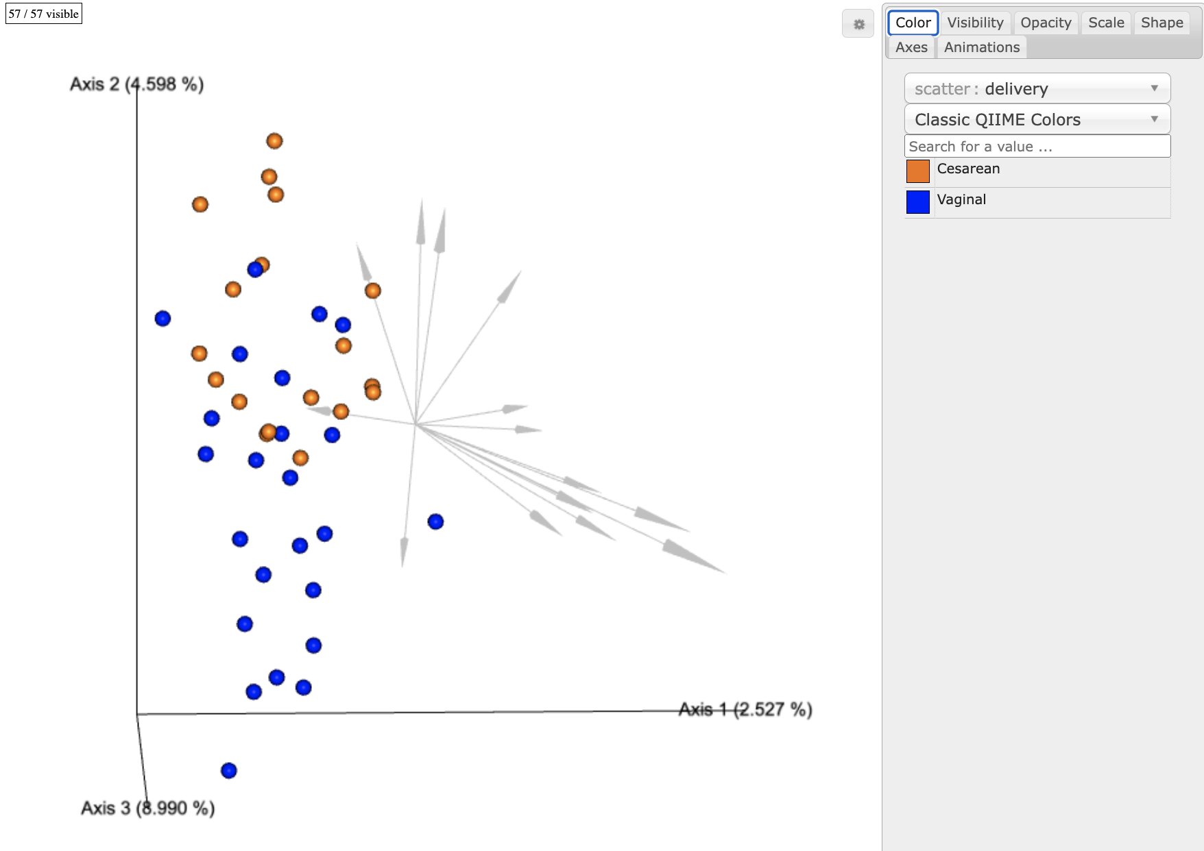
We can also see that the birthmode grouping is separated entirely along the first PC (axis 2). We can now use Qurro to explore the feature loading partitions (arrows) in this biplot as a log-ratio of the original table counts. This allows us to relate these low-dimensional representations back to our original data. Additionally, log-ratios provide a nice set of data points for additional analysis such as LME models.
from qiime2.plugins.qurro.actions import loading_plot

# run Qurro
qurro_plot = loading_plot(tempted_res.individual_biplot, table,
                          metadata,
                          feature_metadata=taxonomy.view(q2.Metadata))
# save visual
qurro_plot.visualization.save('ECAM-Qiita-10249/qurro.qzv')
2961 feature(s) in the BIOM table were not present in the feature rankings.
These feature(s) have been removed from the visualization.
'ECAM-Qiita-10249/qurro.qzv'
From the Qurro output qurro.qzv we will simply choose the PC2 loadings above and below zero as the numerator (red ranks) and denominator (blue ranks) to create a log-ratio that differentiates the samples by birth mode status. Log-ratios can also be chosen by taxonomy or sequence identifiers (see the Qurro tutorials here for more information). We can plot this log-ratio in Qurro with the x-axis as time and the color as birth mode, which clearly shows nice separation between phenotypes.
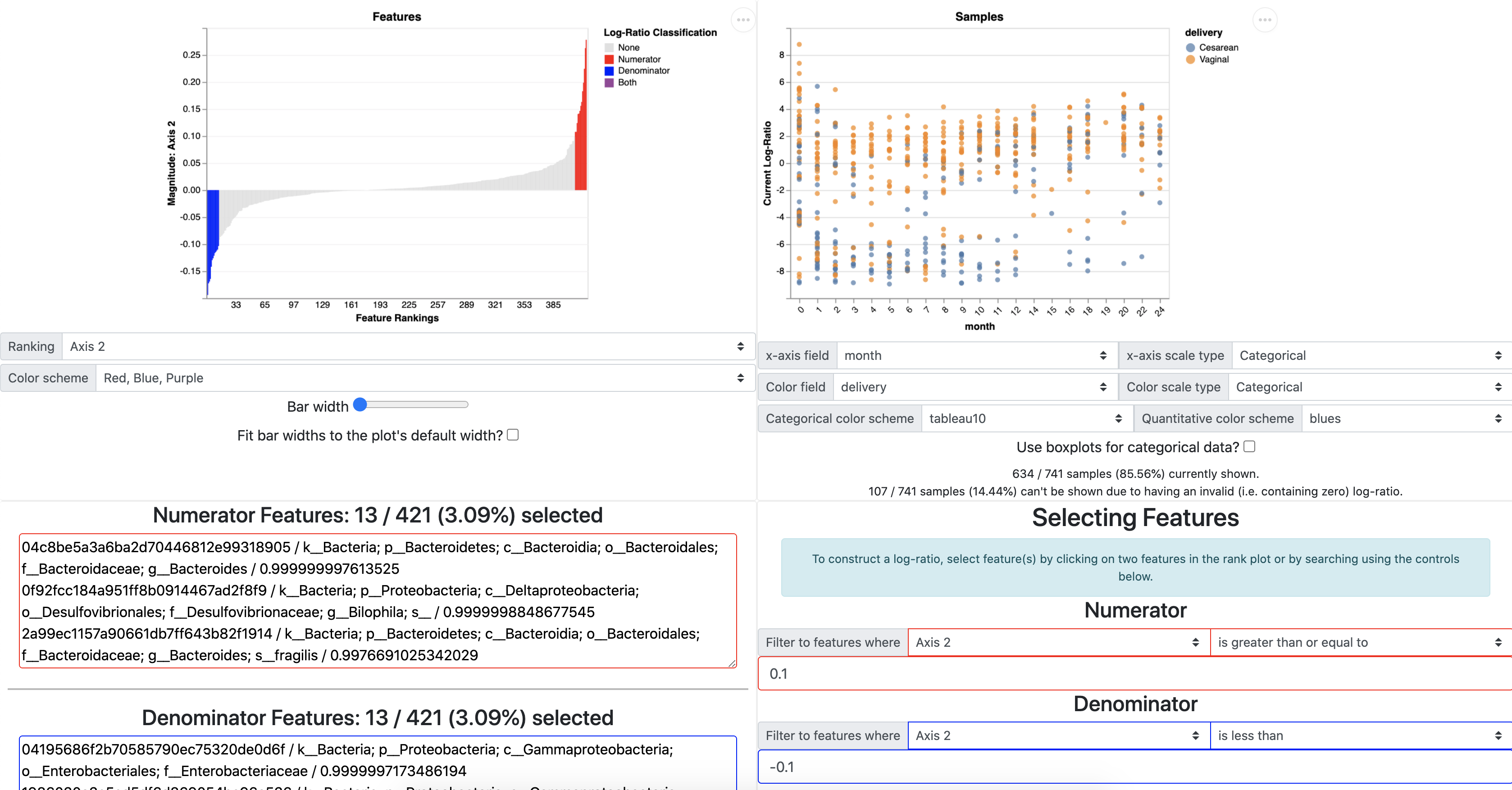
We can further explore these phenotype differences by exporting the sample_plot_data.tsv from Qurro (marked in a orange box above) which will provide the selected log-ratio values for each sample. We can then merge this sample_plot_data with our sample metadata in python or R.
Note: Qurro will have an option to export all of the metadata or only the log-ratio data soon.
import pandas as pd

# import log-ratio data
metadata_one = pd.read_csv('ECAM-Qiita-10249/metadata.tsv',
                           sep='\t', index_col=0)
# import rest of the metadata
metadata_two = pd.read_csv('ECAM-Qiita-10249/sample_plot_data.tsv',
                           sep='\t', index_col=0)[['Current_Log_Ratio']]
# merge the data
log_ratio_metdata = pd.concat([metadata_two, metadata_one], axis=1)
# ensure no duplicate columns
log_ratio_metdata = log_ratio_metdata.dropna(subset=['Current_Log_Ratio'])
log_ratio_metdata.index = log_ratio_metdata.index.astype(str)
# export in QIIME2 format
log_ratio_metdata = log_ratio_metdata[['month','host_subject_id',
                                       'delivery','Current_Log_Ratio']]

log_ratio_metdata.index.name = '#SampleID'
log_ratio_metdata.to_csv('ECAM-Qiita-10249/merged_sample_plot_data.tsv', sep='\t')
log_ratio_metdata.head(2)
| month | host_subject_id | delivery | Current_Log_Ratio | |
|---|---|---|---|---|
| #SampleID | ||||
| 10249.C018.14SS | 16.0 | 18.0 | Vaginal | 1.604457 |
| 10249.C020.22SS | 20.0 | 20.0 | Cesarean | 3.479770 |
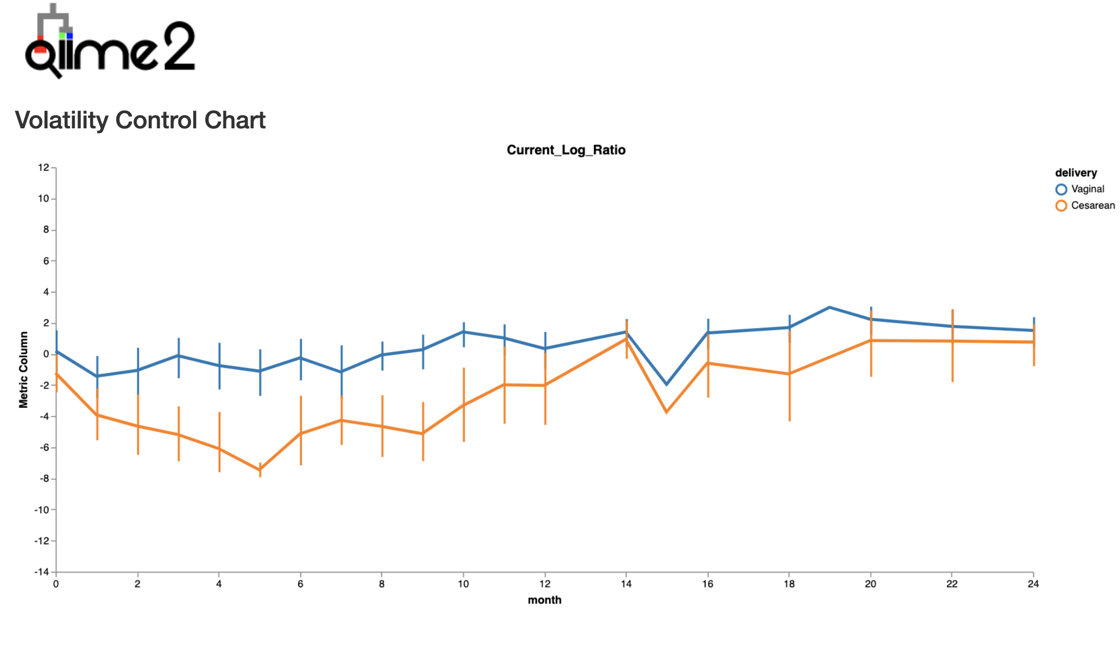
As you can see above the metadata now has the added column of Current_Log_Ratio from Qurro. So now we will continue to explore this log-ratio by first plotting it explicitly over time with q2-longitudinal.
from qiime2.plugins.longitudinal.actions import (volatility, linear_mixed_effects)

# make a time series plot of log-ratio
temporal_plot = volatility(q2.Metadata(log_ratio_metdata),
                           'month',
                           individual_id_column='host_subject_id',
                           default_group_column='delivery',
                           default_metric='Current_Log_Ratio')
temporal_plot.visualization.save('ECAM-Qiita-10249/log_ratio_plot.qzv')
'ECAM-Qiita-10249/log_ratio_plot.qzv'
This demonstrates that we can recreate the separation by birth mode that we saw in both the subject_biplot & state_subject_ordination, allowing us to associate specific taxa (in the numerator or denominator) with a particular phenotype.
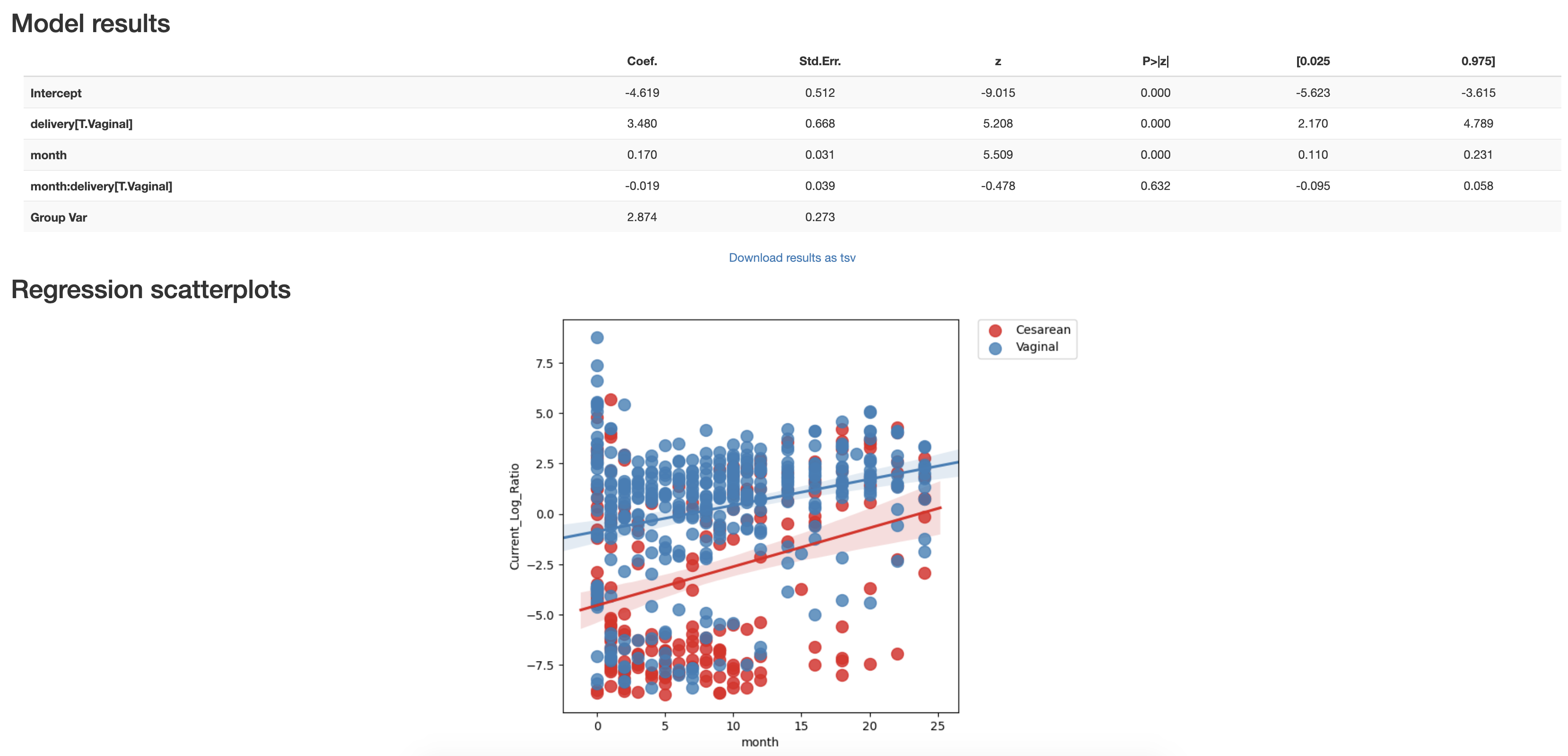
We can test the statistical power of this log-ratio to differentiate samples by birth mode status using a linear mixed effects (LME) through q2-longitudinal.
# Run LME model on log-ratio
lme_plot = linear_mixed_effects(q2.Metadata(log_ratio_metdata),
                                'month',
                                individual_id_column='host_subject_id',
                                group_columns='delivery',
                                metric='Current_Log_Ratio')
lme_plot.visualization.save('ECAM-Qiita-10249/lme_log_ratio.qzv')
/Users/cameronmartino/miniconda2/envs/qiime2-2019.7/lib/python3.6/site-packages/q2_longitudinal/_longitudinal.py:291: UserWarning: This is only a warning, and the results of this action are still valid. The column name "predicted Current_Log_Ratio" already exists in your metadata file. Any "raw" metadata that can be downloaded from the resulting visualization will contain overwritten values for this metadata column, not the original values.
  warnings.warn(warning, UserWarning)
'ECAM-Qiita-10249/lme_log_ratio.qzv'
From this LME model we can see that indeed the birthmode grouping is significant across time.