This notebook illustrates the Discrete Fourier Transformation (DFT) for different time series.

The coefficients of the DFT are one of the many features in tsfresh.

Some theoretical background¶

If we see a series of length $n$ - without timestamps - we don't have any idea about the time domain: In what time was the series recorded? What is the timedelta between 2 observations? The only thing we know (or, more realistic, assume) is that the series is uniformly sampled through time. Of course, with the knowledge of the sampling frequency, one can draw conclusions about the real frequencies in the time domain. But tsfresh does not incorporate this information.

Therefore, in Discrete Fourier Transform (DFT), "frequencies" are expressed in terms of "fractions of series length", $2\pi k/n$, $k=0, ..., n-1$. One can read it as "$2\pi k$ divided on $n$ points" or "$k$ periods of length $2\pi$ divided on $n$ points" or "$k$ cycles among $n$ points". At "time" $m \in \lbrace0, ..., n-1\rbrace$, the value $a_m$ is observed.

The definition used in the implementation in np.fft is (picture from numpy docs): $Definition in implementation np.fft$

with $a_m$ being the (possibly complex) value of the series at position $m$ and the series length $n$. $a_m$ is multiplied with the complex number on the angle $2\pi k m/n$ (in rad not deg measure) on the unit circle. The following picture shows how the complex exponential function rotates among the unit circle / shows "Euler's Theorem" (figure taken from Wikipedia):

The resulting coefficients $A_k$ can be drawn on a complex pane, too (figure from Wikipedia):

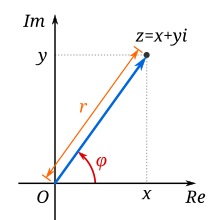
The absolute value $r$ of the complex DFT coefficient corresponds to the amplitude of the oscillation, and the angle $\phi$ corresponds to the phase.

It is stated in Wikipedia (Notation is modified):

It's amplitude and phase are

$|A_k|$ / $n $ and $arctan(Im(A_k), Re(A_k))$

Note the normalization of the Amplitude with the series length $n$.

In [1]:

import numpy as np
import matplotlib.pylab as plt
import seaborn as sns
import pandas as pd
from numpy.fft import rfft
sns.set_style("whitegrid")
sns.set_palette('colorblind')

In [2]:

def plot_x_and_rfft(x, fft_coeffs):
    fft = fft_coeffs
    plt.figure(figsize=(12, 4))
    
    plt.subplot(211)
    plt.title("Time Series")
    plt.plot(x)
    
    plt.subplot(212)
    plt.plot(fft.real, label="real", marker="o")
    plt.plot(fft.imag, label="imag", marker="o")
    plt.plot(np.abs(fft), label="abs", marker="o")
    plt.title("Real, imaginary and absolute part of DFT coefficients A(k)")
    plt.legend()
    
    plt.tight_layout()
    plt.show()

Compose a Signal With up to 14 Periods of Cos Included¶

Let's compose a series as the sum of some cosine waves with different frequencies.

In [3]:

n = 200  # no of samples
m = np.linspace(0, 1, n, endpoint=False)  # the results differ with the defaul endpoint=True
x = np.zeros(n)
plt.figure(figsize=(20,20))
for i in range(15):
    plt.subplot(5, 3, i+1)
    # the results differ with the defaul endpoint=True
    cos_wave = np.cos(np.linspace(0, i*2*np.pi, n, endpoint=False))
    plt.title("Signal no {}: {} Cos-Waves".format(i,i))
    plt.plot(cos_wave)
    x = x + cos_wave
plt.show()

The analytical solution of the DFT is:

Amplitude (i.e. absolute value) is 1 for the first 15 coefficients
angle, i.e. phase, should be 0 deg for the first 15 coefficients

In [4]:

fft_coeffs = rfft(x)
amp_deg = tuple(zip(range(20), np.abs(fft_coeffs)[:20], np.angle(fft_coeffs, deg=True)[:20]))
print("No \t Abs.Value \t Abs.Value/N \t angle in deg")
for no, amp, deg in amp_deg:
    print("{:d} \t {:f} \t {:f} \t {:4.2f}".format(no, amp, amp / n, deg))

No 	 Abs.Value 	 Abs.Value/N 	 angle in deg
0 	 200.000000 	 1.000000 	 0.00
1 	 100.000000 	 0.500000 	 0.00
2 	 100.000000 	 0.500000 	 -0.00
3 	 100.000000 	 0.500000 	 -0.00
4 	 100.000000 	 0.500000 	 0.00
5 	 100.000000 	 0.500000 	 -0.00
6 	 100.000000 	 0.500000 	 -0.00
7 	 100.000000 	 0.500000 	 -0.00
8 	 100.000000 	 0.500000 	 0.00
9 	 100.000000 	 0.500000 	 -0.00
10 	 100.000000 	 0.500000 	 -0.00
11 	 100.000000 	 0.500000 	 -0.00
12 	 100.000000 	 0.500000 	 -0.00
13 	 100.000000 	 0.500000 	 0.00
14 	 100.000000 	 0.500000 	 -0.00
15 	 0.000000 	 0.000000 	 -50.74
16 	 0.000000 	 0.000000 	 -120.06
17 	 0.000000 	 0.000000 	 -47.79
18 	 0.000000 	 0.000000 	 -57.17
19 	 0.000000 	 0.000000 	 -4.00

If you use np.linspace with endpoint=True in the signal generation, you won't get the correct results.

The amplitude for the 0th Fourier coefficient - which corresponds to the constant 1 - is correct. But obviously, all the other amplitudes are wrong. Moreover, they are consistently half of the correct amplitude. Why is this the case?

I won't go into detail here, but it is because the output of the DFT - in case of a real valued elements $a_m$ - is symmetric. This means that an investigated "frequency" is splitted among two values of $k$, and so is the amplitude (not for $k=0$).

Use Normalization to get Amplitude Information¶

There is a difference in the implementations in np.fft and scipy.fftpack: NumPy provides the normalization flag, whereas fftpack does not. But be aware: The normalization does not yield true amplitudes, because the normalization is done by $1 / \sqrt{n}$. Correct amplitudes can be calculated by multiplication with $1/n$. However, this normalization is sufficient to compare timeseries with different length.

In [5]:

print("Unnormalized")
plot_x_and_rfft(x, rfft(x))
print("Normalized with 1 / sqrt(N)")
plot_x_and_rfft(x, rfft(x, norm="ortho"))

Unnormalized

Normalized with 1 / sqrt(N)

For correct resampling via irfft to the time domain, the normalization flag in rfft and irfft must be equal (None or "ortho").

In [6]:

plt.plot(x, '--')
plt.plot(np.fft.irfft(rfft(x, norm="ortho"), norm="ortho"), ':')
plt.legend(['raw', 'resampled'])
plt.show()

Resampling With Coefficients k>=10 Rejected¶

What happens if one tries to resample the signal from the first 10 coefficients only and discard the rest? How does the plot look like?

In [7]:

fft_coeffs = rfft(x, norm="ortho")
trunc_fft_coeffs = np.ones(len(fft_coeffs)) * 0+0j
trunc_fft_coeffs[0:10] = fft_coeffs[0:10]
trunc_fft_coeffs[0:15]  # the remaining entries are zero

Out[7]:

array([ 14.14213562 +0.00000000e+00j,   7.07106781 +1.93774590e-15j,
         7.07106781 -1.72812614e-15j,   7.07106781 -5.70583545e-15j,
         7.07106781 +4.21786636e-15j,   7.07106781 -3.98762969e-15j,
         7.07106781 -1.21015308e-14j,   7.07106781 -6.01337816e-15j,
         7.07106781 +6.47656704e-15j,   7.07106781 -5.10788198e-15j,
         0.00000000 +0.00000000e+00j,   0.00000000 +0.00000000e+00j,
         0.00000000 +0.00000000e+00j,   0.00000000 +0.00000000e+00j,
         0.00000000 +0.00000000e+00j])

In [8]:

plt.plot(np.fft.irfft(fft_coeffs, norm="ortho"))  # plot resampled with all coefficients
plt.plot(np.fft.irfft(trunc_fft_coeffs, norm="ortho"))  # plot resampled with truncated coefficients
plt.legend(["not truncated", "truncated"])
plt.show()

We see an information loss without these coefficients.

What about a non-integer amount of cycles?¶

Truncate the time series from above. The number of cycles is not integer any more.

In [9]:

y = x[0:-50]  # length is now 150, some periods are not integer any more

In [10]:

print("Unnormalized")
plot_x_and_rfft(y, rfft(y))
print("Normalized with 1 / sqrt(N)")
plot_x_and_rfft(y, rfft(y, norm="ortho"))

Unnormalized

Normalized with 1 / sqrt(N)

About the first 11 coefficients seem to be important. Plot the inverted coefficients / resampled signal.

In [11]:

plt.plot(y, '--')
plt.plot(np.fft.irfft(rfft(y, norm="ortho"), norm="ortho"), ':')
plt.legend(["raw", "resampled"])
plt.show()

We do not have an analytical description of the signal any more, but it seems that it is perfectly described by the DFT coefficients, as it can be resampled without an error.

Signal Corrupted With Noise¶

In [12]:

noise = np.random.normal(loc=0.0, scale=1, size=200)

In [13]:

x_with_noise = x + noise
plt.plot(x_with_noise)
plt.show()

Whoosh, this signal seems corrupted. What are the results of the DFT?

In [14]:

print("Unnormalized")
plot_x_and_rfft(x_with_noise, rfft(x_with_noise))
print("Normalized with 1 / sqrt(N)")
plot_x_and_rfft(x_with_noise, rfft(x_with_noise, norm="ortho"))

Unnormalized

Normalized with 1 / sqrt(N)

With this small amount of noise, one can still see the importance of the first 15 DFT coefficients. With more noise (i.e. a larger stddev), the result gets, unsurprisingly, worse.

Gaussian Noise¶

How is gaussian noise treated by the DFT?

In [15]:

noise = np.random.normal(loc=0.0, scale=1, size=200)

In [16]:

print("Unnormalized")
plot_x_and_rfft(noise, rfft(noise))
print("Normalized")
plot_x_and_rfft(noise, rfft(noise, norm="ortho"))

Unnormalized

Normalized

For a random noise, all coefficients seem to be relevant. There seems to be no pattern.

Polynomial Signal¶

Discrete Fourier Transformation of an arbitrary polynomial series.

In [17]:

z = np.linspace(-1, 1, n, endpoint=False)
polynomial = z + z**2 - z**3 + z**4 - z**5  # some arbitrary composition

In [18]:

print("Unnormalized")
plot_x_and_rfft(polynomial, rfft(polynomial))
print("Normalized with 1 / sqrt(N)")
plot_x_and_rfft(polynomial, rfft(polynomial, norm="ortho"))

Unnormalized

Normalized with 1 / sqrt(N)

Discard all DFT coefficients with k >= 10 and k >= 5 and plot the resampling results.

In [19]:

fft_coeffs = rfft(polynomial, norm="ortho")
trunc_fft_coeffs_10 = np.ones(len(fft_coeffs)) * 0+0j
trunc_fft_coeffs_5 = np.ones(len(fft_coeffs)) * 0+0j
trunc_fft_coeffs_10[0:10] = fft_coeffs[0:10]
trunc_fft_coeffs_5[0:5] = fft_coeffs[0:5]

In [20]:

plt.plot(polynomial)
plt.plot(np.fft.irfft(rfft(polynomial, norm="ortho"), norm="ortho"))
plt.plot(np.fft.irfft(trunc_fft_coeffs_10, norm="ortho"))
plt.plot(np.fft.irfft(trunc_fft_coeffs_5, norm="ortho"))
plt.legend(["raw", "resampled_full", "resampled_k<10", "resampled_k<5"])
plt.show()

Conclusion¶

For k=0, the exponential function reduces to 1 and the coefficient is simply the sum of all series values
The DFT k=1 coefficient correlates the signal to an oscillation with 1 period in the signal, the k=2 coefficient correlates it to an oscillation with 2 periods in the signal, and so on
If you want you can make the statement: Taking the first DFT coefficients corresponds to a lowpass behavior, taking the last DFT coefficients corresponds to a highpass behavior, and you can realize whatever bandpass you want by picking the coefficients of interest
Discrete Fourier Transformation (DFT) is not restricted to obviously periodic signals
If the input signal is real valued, one can exploit the symmetry of the DFT coefficients

Further Research¶

If you are interested in the symmetry of the DFT and the important but unmentioned Nyquist Frequency, you can find many valuable resources in the wild world wide web