From Maps to Models - Tutorials for structural geological modeling using GemPy and GemGIS¶

Example 6 - Planar Dipping Layers¶

This example will show how to convert the geological map below using GemGIS to a GemPy model. This example is based on digitized data. The area is 1370 m wide (W-E extent) and 1561 m high (N-S extent). The vertical model extent varies between 0 m and 800 m. The model represents planar layers dipping towards the southwest.

In this tutorial, you will learn the following:
- How to build your sixth GemPy model with input data generated through GemGIS
- Finishing the the extra model for that section

Your Tasks¶

Georeference the map in QGIS given the dimensions above using the coordinate reference system with the EPSG code 4326
Digitize the layer boundaries (including a formation column) and the topographic lines (including a Z column)
Digitize so-called strike lines for the different layers. The orientations used for GemPy will be calculated from the strike lines.

Contents¶

Installing GemPy and GemGIS
Importing Libraries
Data Preparation
GemPy Model calculation
Model Visualization and Post-Processing
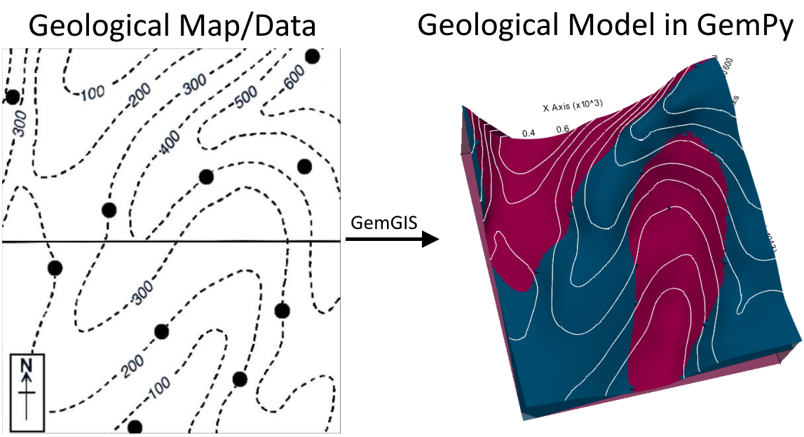1. Visualizing the computed model in 2D
2. Visualizing the computed model in 3D

Source: Powell, D. (1995): Interpretation geologischer Strukturen durch Karten - Eine praktische Anleitung mit Aufgaben und Lösungen, page 23, figure 20 B, Springer Verlag Berlin, Heidelberg, New York, ISBN: 978-3-540-58607-4.

Installing GemPy and GemGIS¶

If you have not installed GemPy yet, please follow the GemPy installation instructions and the GemGIS installation instructions. If you encounter any issues, feel free to open a new discussion at GemPy Discussions or GemGIS Discussions. If you encounter an error in the installation process, feel free to also open an issue at GemPy Issues or GemGIS Issues. There, the GemPy and GemGIS development teams will help you out.

Importing Libraries¶

For this notebook, we need the geopandas library for the data preparation, rasterio for dealing with the created digital elevation model, matplotlib for plotting, numpy for some numerical calculations, pandas for manipulating DataFrames and of course the gempy and gemgis libraries. Any warnings that may appear can be ignored for now. The file path is set to load the data provided for this tutorial.

In [ ]:

import geopandas as gpd
import rasterio
import warnings
warnings.filterwarnings("ignore")
import gemgis as gg
import matplotlib.pyplot as plt
import numpy as np
import gempy as gp
import pyvista as pv
import pandas as pd

In [ ]:

file_path = '../../data/example25_planar_dipping_layers/'

Data Preparation¶

At his point, you should have the topographic contour lines (including a Z column) and the layer boundaries (including a formation column) digitized. If not, please generate the data before continuing with this tutorial.

Creating Digital Elevation Model from Contour Lines¶

The digital elevation model (DEM) will be created by interpolating the contour lines digitized from the georeferenced map using the SciPy Radial Basis Function interpolation wrapped in GemGIS. The respective function used for that is gg.vector.interpolate_raster().

Source: Powell, D. (1995): Interpretation geologischer Strukturen durch Karten - Eine praktische Anleitung mit Aufgaben und Lösungen, page 23, figure 20 B, Springer Verlag Berlin, Heidelberg, New York, ISBN: 978-3-540-58607-4.

Loading contour lines¶

First, the contour lines are loaded using GeoPandas. Please provide here the name of your shape file containing the digitized topographic contour lines.

In [ ]:

topo = gpd.read_file(file_path + 'topo25.shp')
topo.head()

Plotting the contour lines¶

The contour lines are plotted using the built-in plotting function of GeoPandas.

In [ ]:

topo.plot(column='Z', aspect=1, legend=True, cmap='gist_earth')

Interpolating the contour lines¶

The digital elevation model (DEM) will be created by interpolating the contour lines digitized from the georeferenced map using the SciPy Radial Basis Function interpolation wrapped in GemGIS. The respective function used for that is gg.vector.interpolate_raster().

There is also a tutorial available for this task on the GemGIS Documentation page.

In [ ]:

topo_raster = gg.vector.interpolate_raster(gdf=topo, value='Z', method='rbf', res=5)

Plotting the raster¶

The interpolated digital elevation model can be displayed using matplotlib and its plt.imshow() function and by providing the extent of the raster to align it with the contour lines.

In [ ]:

import matplotlib.pyplot as plt

from mpl_toolkits.axes_grid1 import make_axes_locatable

fix, ax = plt.subplots(1, figsize=(5,5))
topo.plot(ax=ax, aspect='equal', column='Z', cmap='gist_earth')
im = ax.imshow(topo_raster, origin='lower', extent=[0,1370,0,1561], cmap='gist_earth')
divider = make_axes_locatable(ax)
cax = divider.append_axes("right", size="5%", pad=0.05)
cbar = plt.colorbar(im, cax=cax)
cbar.set_label('Altitude [m]')
ax.set_xlabel('X [m]')
ax.set_ylabel('Y [m]')

Saving the raster to disc¶

After the interpolation of the contour lines, the raster is saved to disc using gg.raster.save_as_tiff(). The function will not be executed as as raster is already provided with the example data.

Opening Raster¶

The previously computed and saved raster can now be opened using rasterio.

In [ ]:

topo_raster = rasterio.open(file_path + 'raster25.tif')

Processing Stratigraphic Boundaries¶

The interface points will be extracted from LineStrings digitized from the georeferenced map using QGIS. It is important to provide a formation name for each layer boundary. Up until now, only the X and Y position are stored in the vertices of the LineStrings. Using the digital elevation model created already, we will now sample the elevation model at the locations of the vertices to extract the height at this point as the stratigraphic boundary was mapped at the surface.

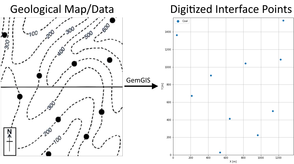Source: Powell, D. (1995): Interpretation geologischer Strukturen durch Karten - Eine praktische Anleitung mit Aufgaben und Lösungen, page 23, figure 20 B, Springer Verlag Berlin, Heidelberg, New York, ISBN: 978-3-540-58607-4.

Opening Stratigraphic Boundaries¶

The stratigraphic units are opened using GeoPandas.

In [ ]:

interfaces = gpd.read_file(file_path + 'interfaces25.shp')
interfaces.head()

Plotting Stratigraphic Boundaries¶

In [ ]:

fig, ax = plt.subplots(1, figsize=(5,5))

interfaces.plot(ax=ax, column='formation', legend=True, aspect='equal')

plt.grid()
ax.set_xlabel('X [m]')
ax.set_ylabel('Y [m]')

Extracting Z coordinates from Digital Elevation Model¶

The vertical position of the interface point will be extracted from the digital elevation model using the GemGIS function gg.vector.extract_xyz(). The resulting GeoDataFrame now contains single points including the information about the respective formation as well as the X, Y, and Z location. This is all we need as preparational steps to generate input data for GemPy.

There is also a tutorial available for this task on the GemGIS Documentation page.

In [ ]:

interfaces_coords = gg.vector.extract_xyz(gdf=interfaces, dem=topo_raster)
interfaces_coords = interfaces_coords.sort_values(by='formation', ascending=False)
interfaces_coords.head()

Plotting the Interface Points¶

The interface points incuding their altitude (Z-) values and the digitized LineString can be plotted using matplotlib.

In [ ]:

fig, ax = plt.subplots(1, figsize=(10,10))

interfaces.plot(ax=ax, column='formation', legend=True, aspect='equal')
interfaces_coords.plot(ax=ax, column='formation', legend=True, aspect='equal')
plt.grid()
plt.xlabel('X [m]')
plt.ylabel('Y [m]')
plt.xlim(0,1370)
plt.ylim(0,1561)

Processing Orientations¶

For this example, orientations must be calculated yourself. They will be calculated using functions implemented in GemGIS and the previously digitized strike lines.

Source: Powell, D. (1995): Interpretation geologischer Strukturen durch Karten - Eine praktische Anleitung mit Aufgaben und Lösungen, page 23, figure 20 B, Springer Verlag Berlin, Heidelberg, New York, ISBN: 978-3-540-58607-4.

Orientations from Strike Lines¶

Strike lines connect outcropping stratigraphic boundaries (interfaces) of the same altitude. In other words: the intersections between topographic contours and stratigraphic boundaries at the surface. The height difference and the horizontal difference between two digitized lines is used to calculate the dip and azimuth and hence an orientation that is necessary for GemPy.

The calculation of orientations from strike lines has been implemented into GemPy for simple cases like these. In order to calculate the orientations, each set of strikes lines/LineStrings for one formation must be given an id number next to the altitude of the strike line. The id field is already predefined in QGIS. The strike line with the lowest altitude gets the id number 1, the strike line with the highest altitude the the number according to the number of digitized strike lines. It is currently recommended to use one set of strike lines for each structural element of one formation as illustrated.

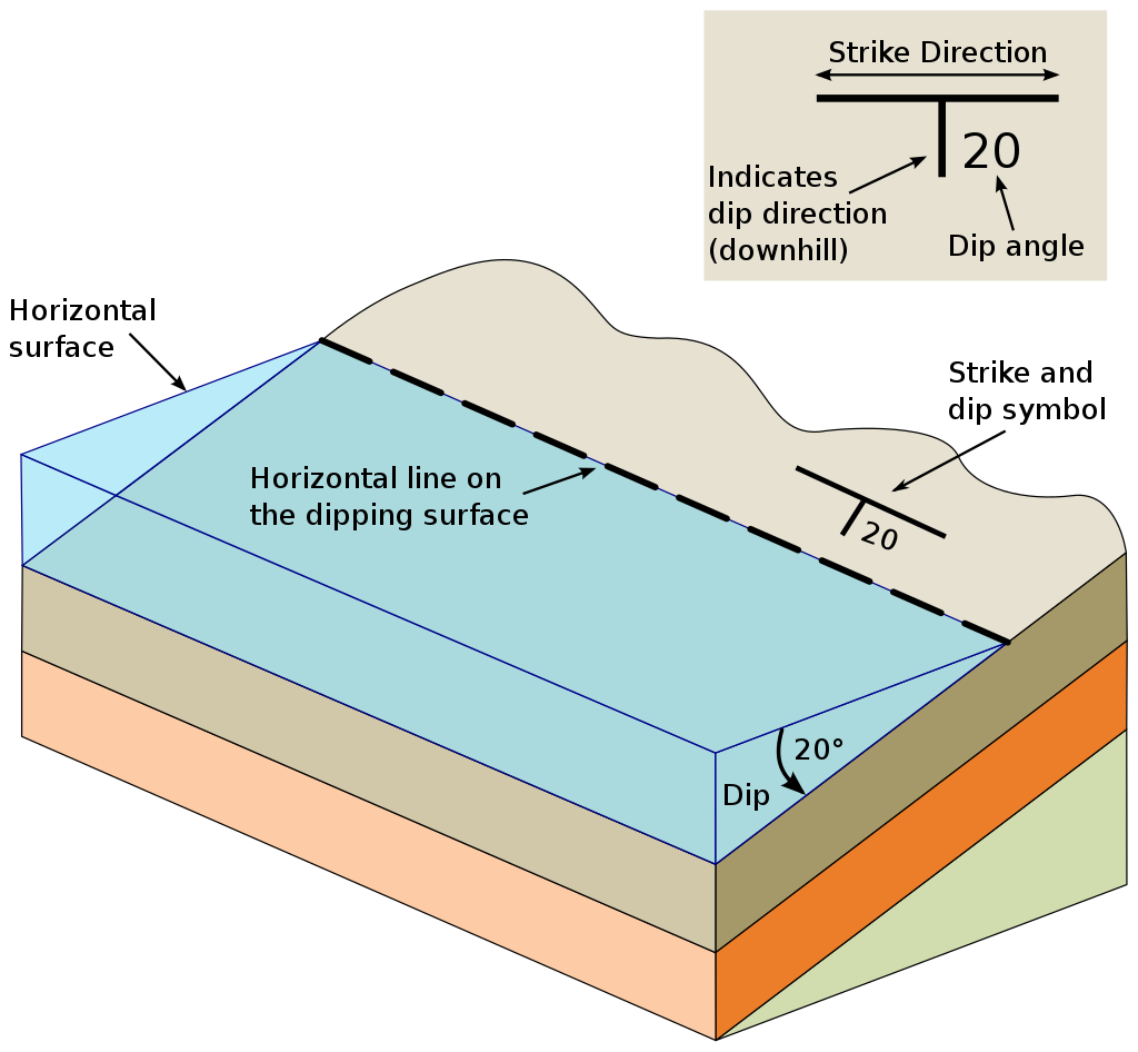
By CrunchyRocks, after Karla Panchuck - https://openpress.usask.ca/physicalgeology/chapter/13-5-measuring-geological-structures/, CC BY 4.0, https://commons.wikimedia.org/w/index.php?curid=113554289

Source: Powell, D. (1995): Interpretation geologischer Strukturen durch Karten - Eine praktische Anleitung mit Aufgaben und Lösungen, page 14, figure 8, Springer Verlag Berlin, Heidelberg, New York, ISBN: 978-3-540-58607-4.

In [ ]:

strikes = gpd.read_file(file_path + 'strikes25.shp')
strikes

Plotting Strike Lines¶

The strike lines can be plotted using matplotlib.

In [ ]:

fig, ax = plt.subplots(1, figsize=(5,5))

strikes.plot(ax=ax,column='id', aspect=1)
interfaces.plot(ax=ax, column='formation', legend=True, aspect='equal')
ax.set_xlabel('X [m]')
ax.set_ylabel('Y [m]')
ax.grid()

Calculate Orientations for each formation¶

The calculations will be calculated using the function gg.vector.calculate_orientations_from_strike_lines() where the strike lines for each single formation will be provided and calculated separately. The result is a GeoDataFrame ready to be used in GemPy.

In [ ]:

orientations_coal = gg.vector.calculate_orientations_from_strike_lines(gdf=strikes[strikes['formation']=='Coal'].sort_values(by='Z', ascending=True).reset_index())
orientations_coal

Merging Orientations for GemPy¶

Since GemPy only takes one DataFrame for the necessary orientations, the single DataFrames are concatenated using pd.concat().

In [ ]:

import pandas as pd
orientations = pd.concat([orientations_coal]).reset_index()
orientations['formation'] = 'Coal'
orientations

Plotting the Orientations¶

The orientations can be plotted using matplotlib.

In [ ]:

fig, ax = plt.subplots(1, figsize=(5,5))

interfaces.plot(ax=ax, column='formation', legend=True, aspect='equal')
interfaces_coords.plot(ax=ax, column='formation', legend=True, aspect='equal')
orientations.plot(ax=ax, color='red', aspect='equal')
plt.grid()
plt.xlabel('X [m]')
plt.ylabel('Y [m]')
plt.xlim(0,1370)
plt.ylim(0,1561)

GemPy Model Calculation¶

The creation of a GemPy Model follows particular steps which will be performed in the following:

Create new model: gp.create_model()
Data Initiation: gp.init_data()
Map Stack to Surfaces: gp.map_stack_to_surfaces()
[...]
Set the Interpolator: gp.set_interpolator()
Computing the Model: gp.compute_model()

Creating the GemPy Model¶

The first step is to create a new empty GemPy model by providing a name for it.

In [ ]:

geo_model = gp.create_model('Model25')
geo_model

Data Initiation¶

During this step, the extent of the model (xmin, xmax, ymin, ymax, zmin, zmax) and the resolution in X, Yand Z direction (res_x, res_y, res_z, equal to the number of cells in each direction) will be set using lists of values.

The interface points (surface_points_df) and orientations (orientations_df) will be passed as pandas DataFrames.

In [ ]:

gp.init_data(geo_model, [0,1370,0,1561,0,800], [100,100,100],
             surface_points_df = interfaces_coords[interfaces_coords['Z']!=0],
             orientations_df = orientations,
             default_values=True)

Inspecting the Surfaces¶

The model consists of five different layers or surfaces now which all belong to the Default series. During the next step, the proper Series will be assigned to the surfaces. Using the surfaces-attribute again, we can check which layers were loaded.

In [ ]:

geo_model.surfaces

Inspecting the Input Data¶

The loaded interface points and orientations can again be inspected using the surface_points- and orientations-attributes. Using the df-attribute of this object will convert the displayed table in a pandas DataFrame.

In [ ]:

geo_model.surface_points.df.head()

In [ ]:

geo_model.orientations.df.head()

Map Stack to Surfaces¶

During this step, the layer of the model is assigned to the Strata1 series. We will also add a Basement here (geo_model.add_surfaces('Basement')).

In [ ]:

gp.map_stack_to_surfaces(geo_model,
                         {
                          'Strata1': ('Coal'),
                         },
                         remove_unused_series=True)
geo_model.add_surfaces('Basement')

Showing the Number of Data Points¶

You can also return the number of interfaces and orientations for each formation using gg.utils.show_number_of_data_points()

In [ ]:

gg.utils.show_number_of_data_points(geo_model=geo_model)

Loading Digital Elevation Model¶

GemPy is capable of including a topography into the modeling process. Here, we use the topography that we have interpolated in one of the previous steps. GemPy takes the file path of the raster/digital elevation model and loads it as grid into the geo_model object.

In [ ]:

geo_model.set_topography(
    source='gdal', filepath=file_path + 'raster25.tif')

Plotting the input data in 2D using Matplotlib¶

The input data can now be visualized in 2D using matplotlib. This might for example be useful to check if all points and measurements are defined the way we want them to. Using the function plot_2d(), we attain a 2D projection of our data points onto a plane of chosen direction (we can choose this attribute to be either 'x', 'y', or 'z').

In [ ]:

gp.plot_2d(geo_model, direction='z', show_lith=False, show_boundaries=False)
plt.grid()

Plotting the input data in 3D using PyVista¶

The input data can also be viszualized using the pyvista package. In this view, the interface points are visible as well as the orientations (marked as arrows) which indicate the normals of each orientation value.

In [ ]:

gp.plot_3d(geo_model, image=False, plotter_type='basic', notebook=True)

Setting the interpolator¶

Once we have made sure that we have defined all our primary information, we can continue with the next step towards creating our geological model: preparing the input data for interpolation.

Setting the interpolator is necessary before computing the actual model. Here, the most important kriging parameters can be defined.

In [ ]:

gp.set_interpolator(geo_model,
                    compile_theano=True,
                    theano_optimizer='fast_compile',
                    verbose=[],
                    update_kriging = False
                    )

Computing the model¶

At this point, we have all we need to compute our full model via gp.compute_model(). By default, this will return two separate solutions in the form of arrays. The first provides information on the lithological formations, the second on the fault network in the model, which is not present in this example.

In [ ]:

sol = gp.compute_model(geo_model, compute_mesh=True)

In [ ]:

sol

In [ ]:

geo_model.solutions

Model Visualization and Post-Processing¶

Visulazing Cross Sections of the computed model¶

Cross sections in different directions and at different cell_numbers can be displayed. Here, we see the folded layers of the model in the different directions.

The first section to be plotted is the custom section Section1 followed by an array of cross sections.

In [ ]:

gp.plot_2d(geo_model, direction=['x', 'x', 'y', 'y'], cell_number=[25,75,25,75], show_topography=True, show_data=False)

Next to the lithology data, we can also plot the calculated scalar field.

In [ ]:

gp.plot_2d(geo_model, direction='y', show_data=False, show_scalar=True, show_lith=False)

Plotting 3D Model¶

In [ ]:

gpv = gp.plot_3d(geo_model, image=False, show_topography=True,
                 plotter_type='basic', notebook=True, show_lith=True)

Conclusions¶

In this tutorial, you have learnt the following:
- How to build your sixth GemPy model with input data generated through GemGIS
- Finishing the the extra model for that section

Outlook¶

In the next tutorial, you will learn the following:
- How to build your fourth GemPy model with input data generated through GemGIS
- How to build a GemPy model with folded layers
- How to obtain the the fold axis of a structure
- How to extract contour lines from a PyVista depth map and to save them as GeoDataFrame
- How to convert a depth map to an array/raster
- How to convert contour lines from that raster

Take me to the next notebook on Github

Source: Bennison, G.M. (1988): An Introduction to Geological Structures and Maps, page 22, figure 9, Springer Verlag Berlin, Heidelberg, New York, ISBN: 978-1-4615-9632-5

Licensing¶

Institute for Computational Geoscience, Geothermics and Reservoir Geophysics, RWTH Aachen University & Fraunhofer IEG, Fraunhofer Research Institution for Energy Infrastructures and Geothermal Systems IEG, Authors: Alexander Juestel. For more information contact: alexander.juestel(at)ieg.fraunhofer.de

All notebooks are licensed under a Creative Commons Attribution 4.0 International License (CC BY 4.0, http://creativecommons.org/licenses/by/4.0/). References for each displayed map are provided. Most of the maps originate from the books of Powell (1992) and Bennison (1990). References for maps with unknown origin will gladly be added.