Visualizing ASPECT unstructured mesh output with yt
In this notebook, we present initial work towards visualizing standard output from the geodynamic code ASPECT in yt.
We demonstrate two methods of loading data first using a simple dataset:
The first method uses the standard yt release, but requires manually loading mesh and field data from .vtu files into memory. The second method is more experimental and uses an early draft of a yt-native frontend for standard ASPECT output available on the aspect branch of the yt fork here.
After that, we show visualizations from a more complex simulation: Visualizing fault formation in the lithosphere
Manual Loading
In order to manually load data, we'll need the standard yt release along with xmltodict and meshio.
pvtu data
The standard ASPECT vtk output is comprised of unstructured mesh data stored in .pvtu files: each .pvtu file is a timestep from the ASPECT simulation and each .pvtu records the .vtu files storing the actual data (when running in parallel, each process will output a .vtu file). So in order to load this data into yt manually, we need to parse our pvtu files to assemble connectivity, coordinatesand node_data arrays and supply them to load_unstructured_mesh function:
import yt
ds = yt.load_unstructured_mesh(
    connectivity,
    coordinates,
    node_data = node_data
)
The following code creates a class to parse a .pvtu file and accompanying .vtu files using a combination of xmltodict and meshio. After instantiating, pvuFile.load() will load each .vtu file into memory as a separate mesh to give to load_unstructured_mesh:
import os
import numpy as np
import xmltodict, meshio

class pvuFile(object):
    def __init__(self,file,**kwargs):
        self.file=file
        self.dataDir=kwargs.get('dataDir',os.path.split(file)[0])
        with open(file) as data:
            self.pXML = xmltodict.parse(data.read())

        # store fields for convenience
        self.fields=self.pXML['VTKFile']['PUnstructuredGrid']['PPointData']['PDataArray']

        self.connectivity = None
        self.coordinates = None
        self.node_data = None

    def load(self):

        conlist=[]  # list of 2D connectivity arrays
        coordlist=[] # global, concatenated coordinate array
        nodeDictList=[] # list of node_data dicts, same length as conlist

        con_offset=-1
        pieces = self.pXML['VTKFile']['PUnstructuredGrid']['Piece']
        if not isinstance(pieces,list):
            pieces = [pieces]

        for mesh_id,src in enumerate(pieces):
            print(f"processing vtu file {mesh_id+1} of {len(pieces)}")
            mesh_name="connect{meshnum}".format(meshnum=mesh_id+1) # connect1, connect2, etc.

            srcFi=os.path.join(self.dataDir,src['@Source']) # full path to .vtu file

            [con,coord,node_d]=self.loadPiece(srcFi,mesh_name,con_offset+1)
            con_offset=con.max()

            conlist.append(con.astype("i8"))
            coordlist.extend(coord.astype("f8"))
            nodeDictList.append(node_d)

        self.connectivity=conlist
        self.coordinates=np.array(coordlist)
        self.node_data=nodeDictList

    def loadPiece(self,srcFi,mesh_name,connectivity_offset=0):
        meshPiece=meshio.read(srcFi) # read it in with meshio
        coords=meshPiece.points # coords and node_data are already global
        cell_type = list(meshPiece.cells_dict.keys())[0]

        connectivity=meshPiece.cells_dict[cell_type] # 2D connectivity array

        # parse node data
        node_data=self.parseNodeData(meshPiece.point_data,connectivity,mesh_name)

        # offset the connectivity matrix to global value
        connectivity=np.array(connectivity)+connectivity_offset

        return [connectivity,coords,node_data]

    def parseNodeData(self,point_data,connectivity,mesh_name):

        # for each field, evaluate field data by index, reshape to match connectivity
        con1d=connectivity.ravel()
        conn_shp=connectivity.shape

        comp_hash={0:'cx',1:'cy',2:'cz'}
        def rshpData(data1d):
            return np.reshape(data1d[con1d],conn_shp)

        node_data={}
        for fld in self.fields:
            nm=fld['@Name']
            if nm in point_data.keys():
                if '@NumberOfComponents' in fld.keys() and int(fld['@NumberOfComponents'])>1:
                    # we have a vector, deal with components
                    for component in range(int(fld['@NumberOfComponents'])):
                        comp_name=nm+'_'+comp_hash[component] # e.g., velocity_cx
                        m_F=(mesh_name,comp_name) # e.g., ('connect1','velocity_cx')
                        node_data[m_F]=rshpData(point_data[nm][:,component])
                else:
                    # just a scalar!
                    m_F=(mesh_name,nm) # e.g., ('connect1','T')
                    node_data[m_F]=rshpData(point_data[nm])

        return node_data
Now lets set a .pvtu solution path then instantiate and load our pvuFile:
DataDir=os.path.join(os.environ.get('ASPECTdatadir','./'),'output_yt_vtu','solution')
pFile=os.path.join(DataDir,'solution-00000.pvtu')
if os.path.isfile(pFile) is False:
    print("data file not found")

pvuData=pvuFile(pFile)
pvuData.load()
processing vtu file 1 of 1
And now let's actually create a yt dataset:
import yt
ds = yt.load_unstructured_mesh(
    pvuData.connectivity,
    pvuData.coordinates,
    node_data = pvuData.node_data,
    length_unit = 'm'
)
yt : [INFO     ] 2020-11-25 15:05:06,275 Parameters: current_time              = 0.0
yt : [INFO     ] 2020-11-25 15:05:06,276 Parameters: domain_dimensions         = [2 2 2]
yt : [INFO     ] 2020-11-25 15:05:06,276 Parameters: domain_left_edge          = [0. 0. 0.]
yt : [INFO     ] 2020-11-25 15:05:06,276 Parameters: domain_right_edge         = [110000. 110000. 110000.]
yt : [INFO     ] 2020-11-25 15:05:06,277 Parameters: cosmological_simulation   = 0.0
Now that we have our data loaded as a yt dataset, we can do some fun things. First, let's check what fields we have:
ds.field_list
[('all', 'T'),
 ('all', 'crust_lower'),
 ('all', 'crust_upper'),
 ('all', 'current_cohesions'),
 ('all', 'current_friction_angles'),
 ('all', 'density'),
 ('all', 'noninitial_plastic_strain'),
 ('all', 'p'),
 ('all', 'plastic_strain'),
 ('all', 'plastic_yielding'),
 ('all', 'strain_rate'),
 ('all', 'velocity_cx'),
 ('all', 'velocity_cy'),
 ('all', 'velocity_cz'),
 ('all', 'viscosity'),
 ('connect1', 'T'),
 ('connect1', 'crust_lower'),
 ('connect1', 'crust_upper'),
 ('connect1', 'current_cohesions'),
 ('connect1', 'current_friction_angles'),
 ('connect1', 'density'),
 ('connect1', 'noninitial_plastic_strain'),
 ('connect1', 'p'),
 ('connect1', 'plastic_strain'),
 ('connect1', 'plastic_yielding'),
 ('connect1', 'strain_rate'),
 ('connect1', 'velocity_cx'),
 ('connect1', 'velocity_cy'),
 ('connect1', 'velocity_cz'),
 ('connect1', 'viscosity')]
as an example of some simple functionality, we can find the min and max values of the whole domain by creating a YTRegion covering the whole domain and selecting the extrema:
ad = ds.all_data()
ad.quantities.extrema(('all','T'))
unyt_array([ 273., 1613.], '(dimensionless)')
creating slice plots is similarlly easy:
slc = yt.SlicePlot(ds,'x',('all','T'))
slc.set_cmap(('all','T'),'hot_r')
slc.set_log('T',False)
yt : [INFO     ] 2020-11-25 15:05:13,952 xlim = 0.000000 110000.000000
yt : [INFO     ] 2020-11-25 15:05:13,952 ylim = 0.000000 110000.000000
yt : [INFO     ] 2020-11-25 15:05:13,953 xlim = 0.000000 110000.000000
yt : [INFO     ] 2020-11-25 15:05:13,954 ylim = 0.000000 110000.000000
yt : [INFO     ] 2020-11-25 15:05:13,954 Making a fixed resolution buffer of (('all', 'T')) 800 by 800

Loading with yt's new ASPECT frontend
An initial draft frontend for ASPECT data is available on the aspect branch of the yt fork at: https://github.com/chrishavlin/yt. Until a PR is submitted and the aspect branch makes its way into the main yt repository, you can clone the fork, checkout the aspect branch and install from source with pip install . At present, you also have to manually install the meshio and xmltodict packages as for the section on Manual Loading.
Once installed, we can load the data using the usual yt method:
import yt
ds = yt.load(pFile)
yt : [INFO     ] 2020-11-25 15:05:29,458 Parameters: current_time              = 0.0
yt : [INFO     ] 2020-11-25 15:05:29,459 Parameters: domain_dimensions         = [1 1 1]
yt : [INFO     ] 2020-11-25 15:05:29,459 Parameters: domain_left_edge          = [0. 0. 0.]
yt : [INFO     ] 2020-11-25 15:05:29,459 Parameters: domain_right_edge         = [100000. 100000. 100000.]
yt : [INFO     ] 2020-11-25 15:05:29,460 Parameters: cosmological_simulation   = 0
yt : [INFO     ] 2020-11-25 15:05:29,486 detected cell type is hexahedron.
slc = yt.SlicePlot(ds,'x',('all','T'))
slc.set_cmap(('all','T'),'hot_r')
slc.show()
yt : [INFO     ] 2020-11-25 15:05:31,123 xlim = 0.000000 100000.000000
yt : [INFO     ] 2020-11-25 15:05:31,124 ylim = 0.000000 100000.000000
yt : [INFO     ] 2020-11-25 15:05:31,125 xlim = 0.000000 100000.000000
yt : [INFO     ] 2020-11-25 15:05:31,125 ylim = 0.000000 100000.000000
yt : [INFO     ] 2020-11-25 15:05:31,126 Making a fixed resolution buffer of (('all', 'T')) 800 by 800

slc.save('figures/aspect_T_slice.png')
yt : [INFO ] 2020-11-25 15:05:33,715 Saving plot figures/aspect_T_slice.png
['figures/aspect_T_slice.png']
slc = yt.SlicePlot(ds,'x',('all','strain_rate'))
slc.set_log('strain_rate',True)
slc.set_cmap(('all','strain_rate'),'kelp')
slc.show()
yt : [INFO     ] 2020-11-25 15:05:34,597 xlim = 0.000000 100000.000000
yt : [INFO     ] 2020-11-25 15:05:34,598 ylim = 0.000000 100000.000000
yt : [INFO     ] 2020-11-25 15:05:34,599 xlim = 0.000000 100000.000000
yt : [INFO     ] 2020-11-25 15:05:34,599 ylim = 0.000000 100000.000000
yt : [INFO     ] 2020-11-25 15:05:34,600 Making a fixed resolution buffer of (('all', 'strain_rate')) 800 by 800

As of now, the field data is not assigned units, so the color axes in these plots are unitless, but we can see we now have the expected units for the axes.
slc.save('figures/aspect_sr_slice.png')
yt : [INFO ] 2020-11-25 15:05:36,144 Saving plot figures/aspect_sr_slice.png
['figures/aspect_sr_slice.png']
A note on higher order elements
ASPECT can output higher order hexahedral elements but at present, yt only supports plotting first order elements. We could truncate the hexahedral elements to the first 8 nodes (the "corner" vertices for a linear element) before loading, but we can actually let yt do that automatically. Since we're using meshio on the back end for parsing the vtu files, however, we'll need a a modified version of meshio as the current vtu support does not include parsing the higher order elements. At present, installing the vtu72 branch of the meshio fork at https://github.com/chrishavlin/meshio will allow yt to load the higher order data (though it will not be used in plotting).
Visualizing fault formation in the lithosphere
The above examples are simple illustrations of loading and slicing ASPECT data with yt, but we can also load more complex ASPECT runs that were run in parallel. Here, we demsonstrate loading a complex simulation investigating fault formation in the lithosphere using the experimental yt-ASPECT loader noted above.
This simulation models lithosphere extension with a pre-existing crustal weak zone. The weak zone is comprised of radomized variation in initial plastic strain, which together with a strain-softening brittle rheology leads to the ermergence of complex faulting networks that accomodate the stretching.
So let's begin by loading up the dataset. This dataset is large -- all the datafiles for a single timestep end up at just over a GB of data, but we only need to load the mesh and connectivity arrays into memory along with the field that we're plotting.
ds = yt.load('aspect/fault_formation/solution-00050.pvtu')
yt : [INFO     ] 2020-11-25 15:06:26,808 Parameters: current_time              = 0.0
yt : [INFO     ] 2020-11-25 15:06:26,808 Parameters: domain_dimensions         = [1 1 1]
yt : [INFO     ] 2020-11-25 15:06:26,809 Parameters: domain_left_edge          = [0. 0. 0.]
yt : [INFO     ] 2020-11-25 15:06:26,809 Parameters: domain_right_edge         = [500000.        500000.        100547.4453125]
yt : [INFO     ] 2020-11-25 15:06:26,810 Parameters: cosmological_simulation   = 0
yt : [INFO     ] 2020-11-25 15:06:28,233 detected cell type is hexahedron.
In these simulations, faults show up most clearly in strain rate, so let's take some slices. Let's start with a vertical slice through the lithosphere:
slc = yt.SlicePlot(ds,'x',('all','strain_rate'))
slc.set_log('strain_rate',True)
slc.set_cmap(('all','strain_rate'),'magma')
slc.hide_axes()
slc.show()
yt : [INFO     ] 2020-11-25 15:07:20,097 xlim = 0.000000 500000.000000
yt : [INFO     ] 2020-11-25 15:07:20,098 ylim = 0.000000 100547.445312
yt : [INFO     ] 2020-11-25 15:07:20,098 xlim = 0.000000 500000.000000
yt : [INFO     ] 2020-11-25 15:07:20,099 ylim = 0.000000 100547.445312
yt : [INFO     ] 2020-11-25 15:07:20,099 Making a fixed resolution buffer of (('all', 'strain_rate')) 800 by 800

Now let's take a horizontal slice at fixed depth within the crust. To do this, we'll adjust provide a center argument to SlicePlot and set it to the domain center in x and y and set the z value to 90% of the maximum height:
c_val = ds.domain_center
c_arr = np.array([c_val[0],c_val[1],ds.domain_width[2]*0.9])
slc = yt.SlicePlot(ds,'z',('all','strain_rate'),center=c_arr)
slc.set_log('strain_rate',True)
slc.set_cmap(('all','strain_rate'),'magma')
slc.hide_axes()
slc.show()
yt : [INFO     ] 2020-11-25 15:07:54,728 xlim = 0.000000 500000.000000
yt : [INFO     ] 2020-11-25 15:07:54,728 ylim = 0.000000 500000.000000
yt : [INFO     ] 2020-11-25 15:07:54,729 xlim = 0.000000 500000.000000
yt : [INFO     ] 2020-11-25 15:07:54,729 ylim = 0.000000 500000.000000
yt : [INFO     ] 2020-11-25 15:07:54,730 Making a fixed resolution buffer of (('all', 'strain_rate')) 800 by 800

This map view shows the complex fault systems arising in this model of lithosphere extension.
3D rendering of aspect data
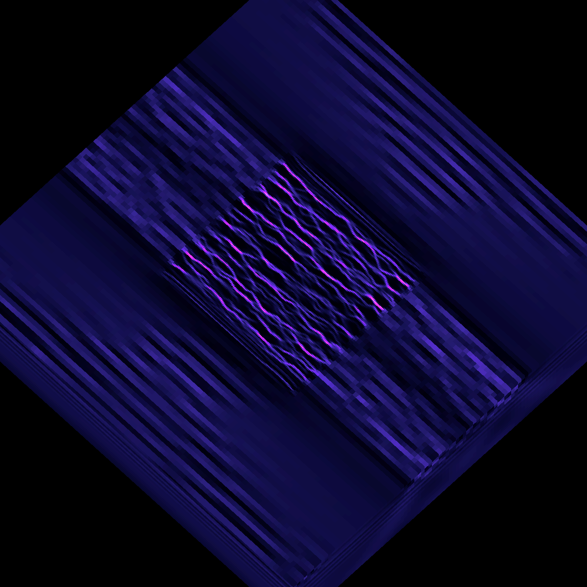
In aspect_mesh_source.py in the code/ folder, we demonstrate how to generate a 3D rendering of ASPECT data following the Unstructured Mesh Rendering documentation. In that script, we use some helper functions (in code/mesh_animator) to set a flight path that moves us around the volume and renders from different angles, including the following view:
The aspect_mesh_source.py script takes some time to run because it's rendering a large number of frames that can be stitched together into an animation. But the starting point to generate 3D renderings is just to create a 3D scene, adjust the view and then render the scene:
import yt

ds = yt.load('aspect/fault_formation/solution-00050.pvtu')
sc = yt.create_scene(ds,('connect1','strain_rate')) # this is the slowest step
We can then pull out the yt MeshSource object and modify the colormap:
ms = sc.get_source()
ms.cmap = 'magma'
ms.color_bounds = (1e-20,1e-14)
And then adjust the camera settings:
cam = sc.camera
new_position = ds.arr([200.0, 200.0, 100.0], 'km')
north_vector = ds.arr([0.0, 0., 0.1], 'dimensionless')
cam.set_position(new_position, north_vector)
cam.set_width(ds.arr([300.0, 300.0, 300.0], 'km'))
To render and save the image, we can just call
sc.save('image_file.png')
Check out this link for the final animation constructed by combining the frames of the flight path generated by code/aspect_mesh_source.py.